Perturbation-response analysis of in silico metabolic dynamics revealed hard-coded responsiveness in the cofactors and network sparsity
Curation statements for this article:-
Curated by eLife

eLife Assessment
This valuable study uses dynamic metabolic models to compare perturbation responses in a bacterial system, analyzing whether they return to their steady state or amplify beyond the initial perturbation. The evidence supporting the emergent properties of perturbed metabolic systems to network topology and sensitivity to specific metabolites is solid.
This article has been Reviewed by the following groups
Discuss this preprint
Start a discussion What are Sciety discussions?Listed in
- Evaluated articles (eLife)
Abstract
Homeostasis is a fundamental characteristic of living systems. Unlike rigidity, homeostasis necessitates that systems respond flexibly to diverse environments. Understanding the dynamics of biochemical systems when subjected to perturbations is essential for the development of a quantitative theory of homeostasis. In this study, we analyze the response of bacterial metabolism to externally imposed perturbations using kinetic models of Escherichia coli ’s central carbon metabolism in nonlinear regimes. We found that three distinct kinetic models consistently display strong responses to perturbations; in the strong responses, minor initial discrepancies in metabolite concentrations from steady-state values amplify over time, resulting in significant deviations. This pronounced responsiveness is a characteristic feature of metabolic dynamics, especially since such strong responses are seldom seen in toy models of the metabolic network. Subsequent numerical studies show that adenyl cofactors consistently influence the responsiveness of the metabolic systems across models. Additionally, we examine the impact of network structure on metabolic dynamics, demonstrating that as the metabolic network becomes denser, the perturbation response diminishes—a trend observed commonly in the models. To confirm the significance of cofactors and network structure, we constructed a simplified metabolic network model underscoring their importance. By identifying the structural determinants of responsiveness, our findings offer implications for bacterial physiology, the evolution of metabolic networks, and the design principles for robust artificial metabolism in synthetic biology and bioengineering.
Article activity feed
-

-
-

eLife Assessment
This valuable study uses dynamic metabolic models to compare perturbation responses in a bacterial system, analyzing whether they return to their steady state or amplify beyond the initial perturbation. The evidence supporting the emergent properties of perturbed metabolic systems to network topology and sensitivity to specific metabolites is solid.
-
Reviewer #1 (Public review):
Summary:
The author studied metabolic networks for central metabolism, focusing on how system trajectories returned to their steady state. To quantify the response, systematic perturbation was performed in simulation and the maximal destabilization away from steady state (compared with initial perturbation distance) was characterized. The author analyzed the perturbation response and found that sparse network and networks with more cofactors are more "stable", in the sense that the perturbed trajectories have smaller deviation along the path back to the steady state.
Strengths and major contributions:
The author compared three metabolic models and performed systematic perturbation analysis in simulation. This is the first work characterized how perturbed trajectories deviate from equilibrium in large …
Reviewer #1 (Public review):
Summary:
The author studied metabolic networks for central metabolism, focusing on how system trajectories returned to their steady state. To quantify the response, systematic perturbation was performed in simulation and the maximal destabilization away from steady state (compared with initial perturbation distance) was characterized. The author analyzed the perturbation response and found that sparse network and networks with more cofactors are more "stable", in the sense that the perturbed trajectories have smaller deviation along the path back to the steady state.
Strengths and major contributions:
The author compared three metabolic models and performed systematic perturbation analysis in simulation. This is the first work characterized how perturbed trajectories deviate from equilibrium in large biochemical systems and illustrated interesting findings about the difference between sparse biological systems and randomly simulated reaction networks.
Discussion and impact for the field:
Metabolic perturbation is an important topic in cell biology and has important clinical implication in pharmacodynamics. The computational analysis in this study provides an initiative for future quantitative analysis on metabolism and homeostasis.
Comments on latest version:
In the latest version of this work, the author included NADH, NADPH into the analysis, and perform some comparison about sensitivity analysis. I think this paper is ready to be finalized, and many open questions inspired from this work can be studied in future.
-
Reviewer #2 (Public review):
The authors have conducted a valuable comparative analysis of perturbation responses in three nonlinear kinetic models of E. coli central carbon metabolism found in the literature. They aimed to uncover commonalities and emergent properties in the perturbation responses of bacterial metabolism. They discovered that perturbations in the initial concentrations of specific metabolites, such as adenylate cofactors and pyruvate, significantly affect the maximal deviation of the responses from steady-state values. Furthermore, they explored whether the network connectivity (sparse versus dense connections) influences these perturbation responses. The manuscript is reasonably well written.
Comments on latest version:
The authors have adequately addressed my concerns.
-
Author response:
The following is the authors’ response to the previous reviews
Reply to the comments of the second referee
We sincerely appreciate the positive evaluation and the useful suggestions on our manuscript.
(1) The authors identified key metabolites affecting responses to perturbations in two ways: (i) by fixing a metabolite's value and (ii) by performing a sensitivity analysis. It would be helpful for the modeling community to understand better the differences and similarities in the obtained results. Do both methods identify substrate-level regulators? Is freezing a metabolite's dynamics dramatically changing the metabolic response (and if yes, which ones are so different in the two cases)? Does the scope of the network affect these differences and similarities?
Thank you for these suggestions. We compared the Sobolʼ …
Author response:
The following is the authors’ response to the previous reviews
Reply to the comments of the second referee
We sincerely appreciate the positive evaluation and the useful suggestions on our manuscript.
(1) The authors identified key metabolites affecting responses to perturbations in two ways: (i) by fixing a metabolite's value and (ii) by performing a sensitivity analysis. It would be helpful for the modeling community to understand better the differences and similarities in the obtained results. Do both methods identify substrate-level regulators? Is freezing a metabolite's dynamics dramatically changing the metabolic response (and if yes, which ones are so different in the two cases)? Does the scope of the network affect these differences and similarities?
Thank you for these suggestions. We compared the Sobolʼ total sensitivity index with the absolute values of the change in the response coefficient (Figure S6 in the revised manuscript). There is no clear relationship between the two quantities. The Sobolʼ sensitivity analysis quantifies how a perturbation on the concentration of a metabolite X contributes to the overall dynamics. On the other hand, the analysis in which metabolitesʼ concentrations are fixed measures how strongly metabolite X helps propagate the perturbations on the other metabolites throughout the metabolic network. In other words, in the Sobolʼ analysis, we evaluate the outcome when the perturbation is applied directly to metabolite X, whereas in the fixing-metabolites analysis, we consider perturbations applied to other metabolites and assess how X influences those perturbations. We believe this conceptual difference explains why the two quantities do not correlate. We suspect that this lack of correlation is independent of the networkʼs scope, because each method evaluates a different aspect of the system. We would say that both methods identify the effect of the metabolite dynamics on the overall dynamics whatever the form is, i.e. the methods do not distinguish the perturbation on the metabolite affecting the overall dynamics by whether the stoichiometric (reactant) way or, the substrate-level regulations. Thus, identifying the substrate-level regulation by utilizing the methods would be challenging.
(2) Regarding the issues the authors encountered when performing the sensitivity analysis, they can be approached in two ways. First, the authors can check the methods for computing conserved moieties nicely explained by Sauro's group (doi:10.1093/bioinformatics/bti800) and compute them for large-scale networks (but beware of metabolites that belong to several conserved pools). Otherwise, the conserved pools of metabolites can be considered as variables in the sensitivity analysis-grouping multiple parameters is a common approach in sensitivity analysis.
Thank you for this helpful suggestion. Following the method described in the reference, we have computed the Sobolʼ sensitivity index of NADH, NADPH, and Q8H2 (with their counterparts algebraically solved and treated as dependent variables). We have updated Figure S5 accordingly.
-
-
eLife Assessment
This valuable study uses dynamic metabolic models to compare perturbation responses in a bacterial system, analyzing whether they return to their steady state or amplify beyond the initial perturbation. The evidence supporting the emergent properties of perturbed metabolic systems to network topology and sensitivity to specific metabolites is solid, although the authors do not explain the origin of some significant inconsistencies between models.
-
Reviewer #1 (Public review):
(1a) Summary:
The author studied metabolic networks for central metabolism, focusing on how system trajectories returned to their steady state. To quantify the response, systematic perturbation was performed in simulation and the maximal destabilization away from steady state (compared with initial perturbation distance) was characterized. The author analyzed the perturbation response and found that sparse network and networks with more cofactors are more "stable", in the sense that the perturbed trajectories have smaller deviation along the path back to the steady state.
(1b) Strengths and major contributions:
The author compared three metabolic models and performed systematic perturbation analysis in simulation. This is the first work characterized how perturbed trajectories deviate from equilibrium in …
Reviewer #1 (Public review):
(1a) Summary:
The author studied metabolic networks for central metabolism, focusing on how system trajectories returned to their steady state. To quantify the response, systematic perturbation was performed in simulation and the maximal destabilization away from steady state (compared with initial perturbation distance) was characterized. The author analyzed the perturbation response and found that sparse network and networks with more cofactors are more "stable", in the sense that the perturbed trajectories have smaller deviation along the path back to the steady state.
(1b) Strengths and major contributions:
The author compared three metabolic models and performed systematic perturbation analysis in simulation. This is the first work characterized how perturbed trajectories deviate from equilibrium in large biochemical systems and illustrated interesting findings about the difference between sparse biological systems and randomly simulated reaction networks.
(1c) Discussion and impact for the field:
Metabolic perturbation is an important topic in cell biology and has important clinical implication in pharmacodynamics. The computational analysis in this study provides an initiative for future quantitative analysis on metabolism and homeostasis.
Comments on revised version:
The revised version of this manuscript made some clarifications, while I think the analysis of response coefficients is still numerical and model-specific, being unclear under dynamical systems of views.
-
Reviewer #2 (Public review):
The authors have conducted a valuable comparative analysis of perturbation responses in three nonlinear kinetic models of E. coli central carbon metabolism found in the literature. They aimed to uncover commonalities and emergent properties in the perturbation responses of bacterial metabolism. They discovered that perturbations in the initial concentrations of specific metabolites, such as adenylate cofactors and pyruvate, significantly affect the maximal deviation of the responses from steady-state values. Furthermore, they explored whether the network connectivity (sparse versus dense connections) influences these perturbation responses. The manuscript is reasonably well written.
Comments on revised version:
The authors have addressed my concerns to a large extent. However, a few minor issues remain, as …
Reviewer #2 (Public review):
The authors have conducted a valuable comparative analysis of perturbation responses in three nonlinear kinetic models of E. coli central carbon metabolism found in the literature. They aimed to uncover commonalities and emergent properties in the perturbation responses of bacterial metabolism. They discovered that perturbations in the initial concentrations of specific metabolites, such as adenylate cofactors and pyruvate, significantly affect the maximal deviation of the responses from steady-state values. Furthermore, they explored whether the network connectivity (sparse versus dense connections) influences these perturbation responses. The manuscript is reasonably well written.
Comments on revised version:
The authors have addressed my concerns to a large extent. However, a few minor issues remain, as listed below:
(1) The authors identified key metabolites affecting responses to perturbations in two ways: (i) by fixing a metabolite's value and (ii) by performing a sensitivity analysis. It would be helpful for the modeling community to understand better the differences and similarities in the obtained results. Do both methods identify substrate-level regulators? Is freezing a metabolite's dynamics dramatically changing the metabolic response (and if yes, which ones are so different in the two cases)? Does the scope of the network affect these differences and similarities?
(2) Regarding the issues the authors encountered when performing the sensitivity analysis, they can be approached in two ways. First, the authors can check the methods for computing conserved moieties nicely explained by Sauro's group (doi:10.1093/bioinformatics/bti800) and compute them for large-scale networks (but beware of metabolites that belong to several conserved pools). Otherwise, the conserved pools of metabolites can be considered as variables in the sensitivity analysis-grouping multiple parameters is a common approach in sensitivity analysis.
-
Author response:
The following is the authors’ response to the original reviews.
Reviewer #1 (Public Reviews):
First, the metabolic network in this study is incomplete. For example, amino acid synthesis and lipid synthesis are important for biomass and growth, but they4 are not included in the three models used in this study. NADH and NADPH are as important as ATP/ADP/AMP, but they are not included in the models. In the future, a more comprehensive metabolic and biosynthesis model is required.
Thank you for the critical comment on the weakness of the present study. We actually tried to study a larger model like Turnborg et al (2021), which is a model of JCVI-syn3A, but we give up to include it in our model list to study in depth. This is because we noticed that the concentration of ATP in the model can be negative (we confirmed this …
Author response:
The following is the authors’ response to the original reviews.
Reviewer #1 (Public Reviews):
First, the metabolic network in this study is incomplete. For example, amino acid synthesis and lipid synthesis are important for biomass and growth, but they4 are not included in the three models used in this study. NADH and NADPH are as important as ATP/ADP/AMP, but they are not included in the models. In the future, a more comprehensive metabolic and biosynthesis model is required.
Thank you for the critical comment on the weakness of the present study. We actually tried to study a larger model like Turnborg et al (2021), which is a model of JCVI-syn3A, but we give up to include it in our model list to study in depth. This is because we noticed that the concentration of ATP in the model can be negative (we confirmed this with one of the authors of the paper). Another "big" kinetic model of metabolism that we could list would be Khodayari et al (2017). However, we could not find the models to compare the dynamics of this big model with. Therefore, we decided to use the model only for the central carbon metabolism for now. We would like to leave a more extended study for the near future.
We would like to mention that NADH and NADPH are included in Khodayari model and Boecker model, while NADH and NADPH are ramped up to NADH in the latter model.
Second, this work does not provide a mathematical explanation of the perturbation response χ. Since the perturbation analysis is performed close to the steady state (or at least belongs to the attractor of single-steady-state), local linear analysis would provide useful information. By complementing with other analysis in dynamical systems (described below) we can gain more logical insights about perturbation response.
We tried a linear stability analysis. However, with the perturbation strength we used here, the linearization of the model is no longer valid, in the sense that the linearized model
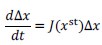
leads to negative concentrations of the metabolites (xst+Δx < 0 for some metabolites). We have added a scatter plot of the response coefficient of trajectories sharing the initial condition, while the dynamics are computed by the original model and the linearized model, respectively. (Fig. S1).
Since the response coefficient is based on the logarithm of the concentrations, as the metabolite concentrations approach zero, the response coefficient becomes larger. The high response coefficient in the Boecker and Chassagnole model would be explained by this artifact. The linearized Khodayari model shows either χ~1 or χ = 0 (one or more metabolite concentrations become negative). This could be due to the number of variables in the model. For the response coefficient to have a larger value, the perturbation should be along the eigenvector that leads to oscillatory dynamics with long relaxation time (i.e., the corresponding eigenvalue has a small real part in terms of absolute value and a non-zero imaginary part). However, since the Khodayari model has about 800 variables, if perturbations are along such directions, there is a high probability that one or more metabolite concentrations will become negative.
We fully agree that if the perturbations on the metabolite concentrations are in the linear regime, the response to the perturbations can be estimated by checking the eigenvalues and eigenvectors. However, we would say that the relationship between the linearized model (and thus the spectrum of eigenvalues) and the original model is unclear in this regime. We remarked this in Lines 158160.
Recommendations for the authors:
My major suggestion is about understanding the key quantity in this study: the response coefficient χ. When the perturbed state is close to the fixed point, one could adopt local stability analysis and consider the linearized system. For a linear system with one stable fixed point P, we consider the Jacobian matrix M on P. If all eigenvalues of M are real and negative, the perturbed trajectory will return to P with each component monotonically varies. If some eigenvalues have negative real part and nonzero imaginary part, then the perturbed trajectory will spiral inward to the fixed point. Depending on the spiral trajectory and the initially perturbed state, some components would deviate furthermore (transiently) from the fixed point on the spiral trajectory. This explains why the response coefficient χ can be greater than 1.
Mathematically, a locally linearized system has similar behavior to the linear system, and the examples in this study can be analyzed in the similar way. Specifically, if a system has many complex eigenvalues, then the perturbed trajectory is more likely to have further deviation. The metabolic network models investigated in this work are not extremely large, and hence the author could analyze its spectrum of the Jacobian matrix at the steady state. Since the steady state is stable, I expect the spectrum located in the left half of the complex plane. If the spectrum spread out away from the real axis, we expect to see more spiral trajectories under perturbation. I think the spectrum analysis will provide a complementary view with respect to analysis on χ. The authors' major findings, about the network sparsity and cofactors, can also be investigated under the framework of the spectrum analysis.
Of course, when the nonlinear system is perturbed far away from the fixed point, there are other geometrical properties of the vector field that can cause the response coefficient χ to be greater than 1. This could also be investigated in the future by testing the behavior of small and large perturbations and observing if the systems have signatures of nonlinearity.
Since all perturbed states return to the steady state, the eigenvalues of the Jacobi matrix accompanying the linearized system around the steady state are in the left half complex plane (negative real value). Also, some eigenvalues have non-zero imaginary parts.
The reason we emphasize the "nonlinear regime" is that the linearization is no longer valid in this regime, i.e. the metabolite concentrations can be negative when we calculate the linearized system. Certainly, there are complex eigenvalues in the Jacobi matrix of any model. However, we would say that there is no clear relationship between the eigenvalues and the response coefficient.
Minor suggestions:
Line 127: Regarding the source of perturbation, cell division also generates unequal concentration of proteins and metabolites for two daughter cells, and it is an interesting mechanism to create metabolic perturbation.
Thank you for the insightful suggestion. We mentioned the cell division as another source of perturbation (Lines 130-131).
Line 175: I do not quite understand the statement "fixing each metabolite concentration...", since the metabolite concentration in the ODE simulation would change immediately after this fixing.
We meant in the sentence that we fixed the concentration of the selected metabolite as the steady state concentration and set the dx/dt of that metabolite to zero. We have rewritten the sentences to avoid confusion (Lines 180-181).
Figure 2: There are a lot of inconsistencies between the three models. Could we learn which model is more reasonable, or the conclusion here is that the cellular response under perturbation is model-specific? The latter explanation may not be quite satisfactory since we expect the overall cellular property should not be sensitive to the model details.
Ideally, the overall cellular property should be insensitive to model details. However, the reality is that the behavior of the models (e.g., steady-state properties, relaxation dynamics, etc.) depends on the specific parameter choices, including what regulation is implemented. I think this situation is part of the motivation for the ensemble modeling (by J. Liao and colleague) that has been developed.
Detailed responsiveness would be model specific. For example, FBP has a fairly strong effect in the Boecker model, but less so in the Khodayari model, and the opposite effect in the Chassagnole model (Fig. 2). Our question was whether there are common tendencies among kinetic models that tend to show model-specific behavior.
Reviewer 2 (Public Review):
(1) In the study on determining key metabolites affecting responses to perturbations (starting from line 171), the authors fix the values of individual concentrations to their steady-state values and observe the responses. Such a procedure adds artificial constraints to the network because, in the natural responses of cells (and models) to perturbations, it is highly unlikely that metabolites will not evolve in time. By fixing the values of specific metabolites, the authors prohibit the metabolic network from evolving in the most optimal way to compensate for the perturbation. Instead of this procedure, have the authors considered for this task applying techniques from variance-based sensitivity analysis (Sobol, global sensitivity analysis), where they can calculate the first-order sensitivity index and total effect index? Using this technique, the authors would be able to determine the key metabolites while allowing for metabolic responses to perturbations without unnatural constraints.
Thank you for the useful suggestion for studying the roles of each metabolite for responsiveness. We have computed the total sensitivity index (Homma and Salteli, 1996) for each metabolite of each model (Fig.S5). The total sensitivity indices of ATP are high-ranked in Khodayari- and Chassagnole model, while it is middle-ranked in the Boecker model. We believe that the importance of the adenyl cofactors is highlighted also in terms of the Sobol’ sensitivity analysis (the figure is referred in Lines 193-195).
We have encountered a minor difficulty for computing the sensitivity index. For the computation of the sensitivity index, we need to carry out the following Monte Carlo integral,
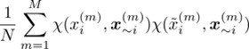
where the superscript (m) is the sample number index. The subscript i represents the ith element of the vector x, and ~i represents the vector x except for the ith element. The tilde stands for resampling.
There are several conserved quantities in each model. For independent resampling, we need to deal with the conserved quantities. For the Boecker and Chassagnole models, we picked a single metabolite from each conservation law and solved its concentration algebraically to make the metabolite concentration the dependent variable. Then, we can resample the metabolite concentration of one metabolite without changing the concentrations of other metabolites, which are independent variables.
However, in the Khodayari model, it was difficult to solve the dependent variables because the model has about 800 variables. Therefore, we gave up the computations of the sensitivity indices of the metabolites whose concentration is part of any conserved quantities, namely NAD, NADH, NADP, NADPH, Q8, and Q8H2.
(2) To follow up on the previous remark, the authors state that the metabolites that augment the response coefficient when their concentration is fixed tend to be allosteric regulators. The authors should report which allosteric regulations are implemented in each of the models so that one can compare against Figure 2. Again, the effect of allosteric regulation by a specific metabolite that is quantified the way the authors did is biased by fixing the concentration value - it is true that negative feedback is broken when the metabolite concentration is fixed, however, in the rate law, there is still the fixed inhibition term with its value corresponding to the inhibition at the steady state. To see the effect of allosteric regulation by a metabolite, one can change the inhibition constants instead of constraining the responses with fixed concentrations.
We have listed the substrate-level regulations (Table S1-3). Also, we re-ran the simulation with reduced the effect of the substrate-level regulations for the reactions that are suspected to influence the change of the response coefficient. Instead of fixing the concentrations (Fig. S6).
The impact of substrate-level regulations is discussed in Lines 203-212.
We replaced "allosteric regulation" with "substrate-level regulation" because we noticed that some regulations are not necessarily allosteric.
(3) Given the role of ATP in metabolic processes, the authors' finding of the sensitivity of the three networks' responses to perturbations in the AXP concentrations seems reasonable. However, drawing such firm conclusions from only three models, with each of them built around one steady state and having one kinetic parameter set despite that they were built for different physiologies, raises some questions. It is well-known in studies related to basins of attraction of the steady states that the nonlinear responses also depend on the actual steady states, the values of kinetic parameters, and implemented kinetic rate law, i.e., not only on the topology of the underlying systems. In the population of only three models, we cannot exclude the possibility of overlaps and strong similarities in the values of kinetic parameters, steady states, and enzyme saturations that all affect and might bias the observed responses. Ideally, to eliminate the possibility of such biases, one should simulate responses of a large population of models for multiple physiologies (and the corresponding steady states) and multiple parameter sets per physiology. This can be a difficult task, but having more kinetic models in this work would go a long way toward more convincing results. Recently, E. coli nonlinear kinetic models from several groups appeared that might help in this task, e.g., Haiman et al., PLoS Comput Biol, 17(1): e1008208, (2021), Choudhury et al., Nat Mach Intell, 4, 710-719, (2022); Hu et al., Metab Eng, 82, 123-133 (2024), Narayanan et al., Nat Commun, 15:723, (2024).
We have computed the responsiveness of 215 models generated by the MASSpy package (Haiman et al, 2021). Several model realizations showed a strong responsiveness, i.e. a broader distribution of the response coefficient (Fig.S8), and mentioned in Lines 339-341.
We would like to mention that the three models studied in the present manuscript have limited overlap in terms of kinetic rate law and, accordingly, parameter values. In the Khodayari model, all reactions are bi-uni or uni-uni reactions implemented by mass-action kinetics, while the Boecker and Chassagnole models use the generalized Michaelis-Menten type rate laws. Also, the relationship between the response coefficients of the original model and the linearized model highlights the differences between the models (Fig. S1). If the models were somewhat effectively similar, the scatter plots of the response coefficient of the original- and linearized model should look similar among the three models. However, the three panels show completely different trends. Thus, the three models have less similarity even when they are linearized around the steady states.
(4) Can the authors share their insights on what could be the underlying reasons for the bimodal distribution in Figure 1E? Even after adding random reactions, the distribution still has two modes - why is that?
We have not yet resolved why only the Khodayari model shows the bimodal distribution of the response coefficient. However, by examining the time courses, the dynamics of the Khodayari model look like those of the excitable systems. This feature may contribute to the bimodal distribution of the response coefficient. In the future, we would like to show whether the system is indeed the excitable system and whcih reactions contribute to such dynamics.
(5) Considering the effects of the sparsity of the networks on the perturbation responses (from line 223 onwards), when we compare the three analyzed models, it is clear that the Khodayari et al. model is a superset of the other two models. Therefore, this model can be considered as, e.g., Chassagnole model with Nadd reactions (though not randomly added). Based on Figures 1b and S2, one can observe that the responses of the Khodayari models have stronger responses, which is exactly opposite to the authors' conclusion that adding the reactions weakens the responses.
The authors should comment on this.
The sparsity of the network is defined by the ratio of the number of metabolites to the number of reactions. Note that the Khodayari model is a superset of the Boecker and Chassagnole models in terms of the number of reactions, but also in terms of the number of metabolites (Boecker does not have the pentose phosphate pathway, Chassagnole does not have the TCA cycle, and neither has oxyative phosphorylation). Thus, even if we manually add reactions to the Boecker model, for example, we cannot obtain a network that is equivalent to the Khodayari model. We added one sentence to clarify the point (Lines 254-255).
Recommendations for the authors:
(1) Some typos: Line 57, remove ?; Line 134, correct "relaxation".
Thank you for pointing out. We fixed the typos.
(2) Lines 510-515, please rewrite/clarify, it is confusing what are you doing.
We rewrote the sentences (Lines 529-532). We are sorry for the confusion.
(3) Line 522, where are the expressions above Leq and K*?
Leq appears in the original paper of the Boecker model, but we decided not to use Leq. We apologize for not removing Leq from the present manuscript. The * in K* is the wildcard for representing the subscripts. We added a description for the role of “*”.
(4) Lines 525-530, based on the wording, it seems like you test first for 128 initial concentrations if the models converge back to the steady state and then you generate another set of 128 initial concentrations - is this what you are doing, or you simply use the 128 initial concentrations that have passed the test?
We apologize for the confusion. We did the first thing. We have rewritten the sentence to make it clearer.
(5) Figure 3, caption, by "broken line," did the authors mean "dashed line"?
We meant dashed line. We changed “broken line” to “dashed line”.
-
-
eLife assessment
This valuable study uses dynamic metabolic models to compare perturbation responses in a bacterial system, analyzing whether they return to their steady state or amplify beyond the initial perturbation. The evidence supporting the emergent properties of perturbed metabolic systems to network topology and sensitivity to specific metabolites is compelling. However, the mathematical explanation of the perturbation response is incomplete, and a more comprehensive metabolic and biosynthesis model would be beneficial.
-
Reviewer #1 (Public Review):
Summary
The author studied metabolic networks for central metabolism, focusing on how system trajectories returned to their steady state. To quantify the response, systematic perturbation was performed in simulation and the maximal destabilization away from the steady state (compared with the initial perturbation distance) was characterized. The author analyzed the perturbation response and found that sparse networks and networks with more cofactors are more "stable", in the sense that the perturbed trajectories have smaller deviations along the path back to the steady state.
Strengths and major contributions
The author compared three metabolic models and performed systematic perturbation analysis in simulation. This is the first work to characterize how perturbed trajectories deviate from equilibrium in …
Reviewer #1 (Public Review):
Summary
The author studied metabolic networks for central metabolism, focusing on how system trajectories returned to their steady state. To quantify the response, systematic perturbation was performed in simulation and the maximal destabilization away from the steady state (compared with the initial perturbation distance) was characterized. The author analyzed the perturbation response and found that sparse networks and networks with more cofactors are more "stable", in the sense that the perturbed trajectories have smaller deviations along the path back to the steady state.
Strengths and major contributions
The author compared three metabolic models and performed systematic perturbation analysis in simulation. This is the first work to characterize how perturbed trajectories deviate from equilibrium in large biochemical systems and illustrated interesting findings about the difference between sparse biological systems and randomly simulated reaction networks.
Weaknesses
There are two main weaknesses in this study:
First, the metabolic network in this study is incomplete. For example, amino acid synthesis and lipid synthesis are important for biomass and growth, but they are not included in the three models used in this study. NADH and NADPH are as important as ATP/ADP/AMP, but they are not included in the models. In the future, a more comprehensive metabolic and biosynthesis model is required.
Second, this work does not provide a mathematical explanation of the perturbation response χ. Since the perturbation analysis is performed close to the steady state (or at least belongs to the attractor of single-steady-state), local linear analysis would provide useful information. By complementing with other analysis in dynamical systems (described below) we can gain more logical insights about perturbation response.
Discussion and impact for the field
Metabolic perturbation is an important topic in cell biology and has important clinical implications in pharmacodynamics. The computational analysis in this study provides an initiative for future quantitative analysis on metabolism and homeostasis.
-
Reviewer #2 (Public Review):
Summary:
The authors have conducted a valuable comparative analysis of perturbation responses in three nonlinear kinetic models of E. coli central carbon metabolism found in the literature. They aimed to uncover commonalities and emergent properties in the perturbation responses of bacterial metabolism. They discovered that perturbations in the initial concentrations of specific metabolites, such as adenylate cofactors and pyruvate, significantly affect the maximal deviation of the responses from steady-state values. Furthermore, they explored whether the network connectivity (sparse versus dense connections) influences these perturbation responses. The manuscript is reasonably well written.
Strengths:
Well-defined and valuable research questions.
Weaknesses:
(1) In the study on determining key metabolites …
Reviewer #2 (Public Review):
Summary:
The authors have conducted a valuable comparative analysis of perturbation responses in three nonlinear kinetic models of E. coli central carbon metabolism found in the literature. They aimed to uncover commonalities and emergent properties in the perturbation responses of bacterial metabolism. They discovered that perturbations in the initial concentrations of specific metabolites, such as adenylate cofactors and pyruvate, significantly affect the maximal deviation of the responses from steady-state values. Furthermore, they explored whether the network connectivity (sparse versus dense connections) influences these perturbation responses. The manuscript is reasonably well written.
Strengths:
Well-defined and valuable research questions.
Weaknesses:
(1) In the study on determining key metabolites affecting responses to perturbations (starting from line 171), the authors fix the values of individual concentrations to their steady-state values and observe the responses. Such a procedure adds artificial constraints to the network because, in the natural responses of cells (and models) to perturbations, it is highly unlikely that metabolites will not evolve in time. By fixing the values of specific metabolites, the authors prohibit the metabolic network from evolving in the most optimal way to compensate for the perturbation. Instead of this procedure, have the authors considered for this task applying techniques from variance-based sensitivity analysis (Sobol, global sensitivity analysis), where they can calculate the first-order sensitivity index and total effect index? Using this technique, the authors would be able to determine the key metabolites while allowing for metabolic responses to perturbations without unnatural constraints.
(2) To follow up on the previous remark, the authors state that the metabolites that augment the response coefficient when their concentration is fixed tend to be allosteric regulators. The authors should report which allosteric regulations are implemented in each of the models so that one can compare against Figure 2. Again, the effect of allosteric regulation by a specific metabolite that is quantified the way the authors did is biased by fixing the concentration value - it is true that negative feedback is broken when the metabolite concentration is fixed, however, in the rate law, there is still the fixed inhibition term with its value corresponding to the inhibition at the steady state. To see the effect of allosteric regulation by a metabolite, one can change the inhibition constants instead of constraining the responses with fixed concentrations.
(3) Given the role of ATP in metabolic processes, the authors' finding of the sensitivity of the three networks' responses to perturbations in the AXP concentrations seems reasonable. However, drawing such firm conclusions from only three models, with each of them built around one steady state and having one kinetic parameter set despite that they were built for different physiologies, raises some questions. It is well-known in studies related to basins of attraction of the steady states that the nonlinear responses also depend on the actual steady states, the values of kinetic parameters, and implemented kinetic rate law, i.e., not only on the topology of the underlying systems. In the population of only three models, we cannot exclude the possibility of overlaps and strong similarities in the values of kinetic parameters, steady states, and enzyme saturations that all affect and might bias the observed responses. Ideally, to eliminate the possibility of such biases, one should simulate responses of a large population of models for multiple physiologies (and the corresponding steady states) and multiple parameter sets per physiology. This can be a difficult task, but having more kinetic models in this work would go a long way toward more convincing results. Recently, E. coli nonlinear kinetic models from several groups appeared that might help in this task, e.g., Haiman et al., PLoS Comput Biol, 17(1): e1008208, (2021), Choudhury et al., Nat Mach Intell, 4, 710-719, (2022); Hu et al., Metab Eng, 82, 123-133 (2024), Narayanan et al., Nat Commun, 15:723, (2024).
(4) Can the authors share their insights on what could be the underlying reasons for the bimodal distribution in Figure 1E? Even after adding random reactions, the distribution still has two modes - why is that?
(5) Considering the effects of the sparsity of the networks on the perturbation responses (from line 223 onwards), when we compare the three analyzed models, it is clear that the Khodayari et al. model is a superset of the other two models. Therefore, this model can be considered as, e.g., Chassagnole model with Nadd reactions (though not randomly added). Based on Figures 1b and S2, one can observe that the responses of the Khodayari models have stronger responses, which is exactly opposite to the authors' conclusion that adding the reactions weakens the responses. The authors should comment on this.
-
-
