A Deep Learning Pipeline for Mapping in situ Network-level Neurovascular Coupling in Multi-photon Fluorescence Microscopy
Curation statements for this article:-
Curated by eLife

eLife Assessment
This work describes a highly complex automated algorithm for analyzing vascular imaging data from two-photon microscopy. This tool has the potential to be extremely valuable to the field and to fill gaps in knowledge of hemodynamic activity across a regional network. The solid biological application provides a demonstration of their pipeline's capabilities and suggests intriguing hypotheses around prolonged vascular tone changes, but will need to be followed up by further experiments to be conclusively demonstrated.
This article has been Reviewed by the following groups
Discuss this preprint
Start a discussion What are Sciety discussions?Listed in
- Evaluated articles (eLife)
Abstract
Functional hyperaemia is a well-established hallmark of healthy brain function, whereby local brain blood flow adjusts in response to a change in the activity of the surrounding neurons. Although functional hyperemia has been extensively studied at the level of both tissue and individual vessels, vascular network-level coordination remains largely unknown. To bridge this gap, we developed a deep learning-based computational pipeline that uses two-photon fluorescence microscopy images of cerebral microcirculation to enable automated reconstruction and quantification of the geometric changes across the microvascular network, comprising hundreds of interconnected blood vessels, pre and post-activation of the neighbouring neurons. The pipeline’s utility was demonstrated in the Thy1-ChR2 optogenetic mouse model, where we observed network-wide vessel radius changes to depend on the photostimulation intensity, with both dilations and constrictions occurring across the cortical depth, at an average of 16.1±14.3 μm (mean±stddev) away from the most proximal neuron for dilations; and at 21.9±14.6 μm away for constrictions. We observed a significant heterogeneity of the vascular radius changes within vessels, with radius adjustment varying by an average of 24 ± 28% of the resting diameter, likely reflecting the heterogeneity of the distribution of contractile cells on the vessel walls. A graph theory-based network analysis revealed that the assortativity of adjacent blood vessel responses rose by 152 ± 65% at 4.3 mW/mm2 of blue photostimulation vs. the control, with a 4% median increase in the efficiency of the capillary networks during this level of blue photostimulation in relation to the baseline. Interrogating individual vessels is thus not sufficient to predict how the blood flow is modulated in the network. Our computational pipeline, to be made openly available, enables tracking of the microvascular network geometry over time, relating caliber adjustments to vessel wall-associated cells’ state, and mapping network-level flow distribution impairments in experimental models of disease.
Article activity feed
-

-
-

eLife Assessment
This work describes a highly complex automated algorithm for analyzing vascular imaging data from two-photon microscopy. This tool has the potential to be extremely valuable to the field and to fill gaps in knowledge of hemodynamic activity across a regional network. The solid biological application provides a demonstration of their pipeline's capabilities and suggests intriguing hypotheses around prolonged vascular tone changes, but will need to be followed up by further experiments to be conclusively demonstrated.
-
Reviewer #1 (Public Review):
Summary:
In this manuscript, the authors describe a new pipeline to measure changes in vasculature diameter upon opt-genetic stimulation of neurons.
The work is interesting and the topic is quite relevant to better understand the hemodynamic response on the graph/network level.
Strengths:
The manuscript provides a pipeline that allows for the detection of changes in the vessel diameter as well as simultaneously allowing for the location of the neurons driven by stimulation.
The resulting data could provide interesting insights into the graph-level mechanisms of regulating activity-dependent blood flow.
The interesting findings include that vessel radius changes depend on depth from the cortical surface and that dilations on average happen closer to the activated neurons.
-
Reviewer #2 (Public Review):
Summary:
The authors develop a highly detailed pipeline to analyze hemodynamic signals from in vivo two-photon fluorescence microscopy. This includes motion correction, segmentation of the vascular network, diameter measurements across time, mapping neuronal position relative to the vascular network, and analyzing vascular network properties (interactions between different vascular segments). For the segmentation, the authors use a Convolution Neural Network to identify vessel (or neural) and background pixels and train it using ground truth images based on semi-automated mapping followed by human correction/annotation. Considerable processing was done on the segmented images to improve accuracy, extract vessel center lines, and compute frame-by-frame diameters. The model was tested with artificial diameter …
Reviewer #2 (Public Review):
Summary:
The authors develop a highly detailed pipeline to analyze hemodynamic signals from in vivo two-photon fluorescence microscopy. This includes motion correction, segmentation of the vascular network, diameter measurements across time, mapping neuronal position relative to the vascular network, and analyzing vascular network properties (interactions between different vascular segments). For the segmentation, the authors use a Convolution Neural Network to identify vessel (or neural) and background pixels and train it using ground truth images based on semi-automated mapping followed by human correction/annotation. Considerable processing was done on the segmented images to improve accuracy, extract vessel center lines, and compute frame-by-frame diameters. The model was tested with artificial diameter increases and Gaussian noise and proved robust to these manipulations.
Network-level properties include Assortativity - a measure of how similar a vessel's response is to nearby vessels - and Efficiency - the ease of flow through the network (essentially, the combined resistance of a path based on diameter and vessel length between two points).
Strengths:
This is a very powerful tool for cerebral vascular biologists as many of these tasks are labor intensive, prone to subjectivity, and often not performed due to the complexity of collecting and managing volumes of vascular signals. Modelling is not my specialty so I cannot speak too specifically, but the model appears to be well-designed and robust to perturbations. It has many clever features for processing the data.
The authors rightly point out that there is a real lack in the field of knowledge of vascular network activity at single-vessel resolution. Network anatomy has been studied, but hemodynamics are typically studied either with coarse resolution or in only one or a few vessels at a time. This pipeline has the potential to change that.
[Editors' note: this work has been through three rounds of revisions, and most recently the authors have added caveats to the discussion. This version of the paper has been assessed by the editors and the weaknesses identified previously remain with earlier versions of the work.]
-
Author response:
The following is the authors’ response to the previous reviews
Reviewer #1 (Public review):
Summary:
In the manuscript the authors describe a new pipeline to measure changes in vasculature diameter upon optogenetic stimulation of neurons. The work is useful to better understand the hemodynamic response on a network /graph level.
Strengths:
The manuscript provides a pipeline that allows to detect changes in the vessel diameter as well as simultaneously allows to locate the neurons driven by stimulation.
The resulting data could provide interesting insights into the graph level mechanisms of regulating activity dependent blood flow.
Weaknesses:
(1) The manuscript contains (new) wrong statements and (still) wrong mathematical formulas.
The symbols in these formulas have been updated to disambiguate them, and the …
Author response:
The following is the authors’ response to the previous reviews
Reviewer #1 (Public review):
Summary:
In the manuscript the authors describe a new pipeline to measure changes in vasculature diameter upon optogenetic stimulation of neurons. The work is useful to better understand the hemodynamic response on a network /graph level.
Strengths:
The manuscript provides a pipeline that allows to detect changes in the vessel diameter as well as simultaneously allows to locate the neurons driven by stimulation.
The resulting data could provide interesting insights into the graph level mechanisms of regulating activity dependent blood flow.
Weaknesses:
(1) The manuscript contains (new) wrong statements and (still) wrong mathematical formulas.
The symbols in these formulas have been updated to disambiguate them, and the accompanying statements have been adjusted for clarity.
(2) The manuscript does not compare results to existing pipelines for vasculature segmentation (opensource or commercial). Comparing performance of the pipeline to a random forest classifier (illastik) on images that are not preprocessed (i.e. corrected for background etc.) seems not a particularly useful comparison.
We’ve now included comparisons to Imaris (a commercial) for segmentation and VesselVio (open-source) for graph extraction software.
For the ilastik comparison, the images were preprocessed prior to ilastik segmentation, specifically by doing intensity normalization.
Example segmentations utilizing Imaris have now been included. Imaris leaves gaps and discontinuities in the segmentation masks, as shown in Supplementary Figure 10. The Imaris segmentation masks also tend to be more circular in cross-section despite irregularities on the surface of the vessels observable in the raw data and identified in manual segmentation. This approach also requires days to months to generate per image stack.
A comparison to VesselVio has now also been generated, and results are visualized in Supplementary Figure 11. VesselVio generates individual graphs for each time point, resulting in potential discrepancies in the structure of the graphs from different time points. Furthermore, Vesselvio uses distance transformation to estimate the vascular radius, which renders the vessel radius estimates highly susceptible to variation in the user selected methodology used to obtain segmentation results; while our approach uses intensity gradient-based boundary detection from centerlines in the image instead mitigating this bias. We have added the following paragraph to the Discussion section on the comparisons with the two methods:
“Comparison with commercial and open-source vascular analysis pipelines
To compare our results with those achievable on these data with other pipelines for segmentation and graph network extraction, we compared segmentation results qualitatively with Imaris version 9.2.1 (Bitplane) and vascular graph extraction with VesselVio [1]. For the Imaris comparison, three small volumes were annotated by hand to label vessels. Example slices of the segmentation results are shown in Supplementary Figure 10. Imaris tended to either over- or under-segment vessels, disregard fine details of the vascular boundaries, and produce jagged edges in the vascular segmentation masks. In addition to these issues with segmentation mask quality, manual segmentation of a single volume took days for a rater to annotate. To compare to VesselVio, binary segmentation masks (one before and one after photostimulation) generated with our deep learning models were loaded into VesselVio for graph extraction, as VesselVio does not have its own method for generating segmentation masks. This also facilitates a direct comparison of the benefits of our graph extraction pipeline to VesselVio. Visualizations of the two graphs are shown in Supplementary Figure 11. Vesselvio produced many hairs at both time points, and the total number of segments varied considerably between the two sequential stacks: while the baseline scan resulted in 546 vessel segments, the second scan had 642 vessel segments. These discrepancies are difficult to resolve in post-processing and preclude a direct comparison of individual vessel segments across time. As the segmentation masks we used in graph extraction derive from the union of multiple time points, we could better trace the vasculature and identify more connections in our extracted graph. Furthermore, VesselVio relies on the distance transform of the user supplied segmentation mask to estimate vascular radii; consequently, these estimates are highly susceptible to variations in the input segmentation masks.We repeatedly saw slight variations between boundary placements of all of the models we utilized (ilastik, UNet, and UNETR) and those produced by raters. Our pipeline mitigates this segmentation method bias by using intensity gradient-based boundary detection from centerlines in the image (as opposed to using the distance transform of the segmentation mask, as in VesselVio).”
(3) The manuscript does not clearly visualize performance of the segmentation pipeline (e.g. via 2d sections, highlighting also errors etc.). Thus, it is unclear how good the pipeline is, under what conditions it fails or what kind of errors to expect.
On reviewer’s comment, 2D slices have been added in the Supplementary Figure 4.
(4) The pipeline is not fully open-source due to use of matlab. Also, the pipeline code was not made available during review contrary to the authors claims (the provided link did not lead to a repository). Thus, the utility of the pipeline was difficult to judge.
All code has been uploaded to Github and is available at the following location: https://github.com/AICONSlab/novas3d
The Matlab code for skeletonization is better at preserving centerline integrity during the pruning of hairs from centerlines than the currently available open-source methods.
- Generalizability: The authors addressed the point of generalizability by applying the pipeline to other data sets. This demonstrates that their pipeline can be applied to other data sets and makes it more useful. However, from the visualizations it's unclear to see the performance of the pipeline, where the pipelines fails etc. The 3d visualizations are not particularly helpful in this respect . In addition, the dice measure seems quite low, indicating roughly 20-40% of voxels do not overlap between inferred and ground truth. I did not notice this high discrepancy earlier. A thorough discussion of the errors appearing in the segmentation pipeline would be necessary in my view to better assess the quality of the pipeline.
2D slices from the additional datasets have been added in the Supplementary Figure 13 to aid in visualizing the models’ ability to generalize to other datasets.
The dice range we report on (0.7-0.8) is good when compared to those (0.56-86) of 3D segmentations of large datasets in microscopy [2], [3], [4], [5], [6]. Furthermore, we had two additional raters segment three images from the original training set. We found that the raters had a mean inter class correlation of 0.73 [7]. Our model outperformed this Dice score on unseen data: Dice scores from our generalizability tests on C57 mice and Fischer rats on par or higher than this baseline.
Reviewer #2 (Public review):
The authors have addressed most of my concerns sufficiently. There are still a few serious concerns I have. Primarily, the temporal resolution of the technique still makes me dubious about nearly all of the biological results. It is good that the authors have added some vessel diameter time courses generated by their model. But I still maintain that data sampling every 42 seconds - or even 21 seconds - is problematic. First, the evidence for long vascular responses is lacking. The authors cite several papers:
Alarcon-Martinez et al. 2020 show and explicitly state that their responses (stimulus-evoked) returned to baseline within 30 seconds. The responses to ischemia are long lasting but this is irrelevant to the current study using activated local neurons to drive vessel signals.
Mester et al. 2019 show responses that all seem to return to baseline by around 50 seconds post-stimulus.
In Mester et al. 2019, diffuse stimulations with blue light showed a return to baseline around 50 seconds post-stimulus (cf. Figure 1E,2C,2D). However, focal stimulations where the stimulation light is raster scanned over a small region focused in the field of view show longer-lasting responses (cf. Figure 4) that have not returned to baseline by 70 seconds post-stimulus [8]. Alarcon-Martinez et al. do report that their responses return baseline within 30 seconds; however, their physiological stimulation may lead to different neuronal and vessel response kinetics than those elicited by the optogenetic stimulations as in current work.
O'Herron et al. 2022 and Hartmann et al. 2021 use opsins expressed in vessel walls (not neurons as in the current study) and directly constrict vessels with light. So this is unrelated to neuronal activity-induced vascular signals in the current study.
We agree that optogenetic activation of vessel-associated cells is distinct from optogenetic activation of neurons, but we do expect the effects of such perturbations on the vasculature to have some commonalities.
There are other papers including Vazquez et al 2014 (PMID: 23761666) and Uhlirova et al 2016 (PMID: 27244241) and many others showing optogenetically-evoked neural activity drives vascular responses that return back to baseline within 30 seconds. The stimulation time and the cell types labeled may be different across these studies which can make a difference. But vascular responses lasting 300 seconds or more after a stimulus of a few seconds are just not common in the literature and so are very suspect - likely at least in part due to the limitations of the algorithm.
The photostimulation in Vazquez et al. 2014 used diffuse photostimulation with a fiberoptic probe similar to Mester et al. 2019 as opposed to raster scanning focal stimulation we used in this study and in the study by Mester et al. 2019 where we observed the focal photostimulation to elicited longer than a minute vascular responses. Uhlirova et al. 2016 used photostimulation powers between 0.7 and 2.8 mW, likely lower than our 4.3 mW/mm2 photostimulation. Further, even with focal photostimulation, we do see light intensity dependence of the duration of the vascular responses. Indeed, in Supplementary Figure 2, 1.1 mW/mm2 photostimulation leads to briefer dilations/constrictions than does 4.3 mW/mm2; the 1.1 mW/mm2 responses are in line, duration wise, with those in Uhlirova et al. 2016.
Critically, as per Supplementary Figure 2, the analysis of the experimental recordings acquired at 3-second temporal resolution did likewise show responses in many vessels lasting for tens of seconds and even hundreds of seconds in some vessels.
Another major issue is that the time courses provided show that the same vessel constricts at certain points and dilates later. So where in the time course the data is sampled will have a major effect on the direction and amplitude of the vascular response. In fact, I could not find how the "response" window is calculated. Is it from the first volume collected after the stimulation - or an average of some number of volumes? But clearly down-sampling the provided data to 42 or even 21 second sampling will lead to problems. If the major benefit to the field is the full volume over large regions that the model can capture and describe, there needs to be a better way to capture the vessel diameter in a meaningful way.
In the main experiment (i.e. excluding the additional experiments presented in the Supplementary Figure 2 that were collected over a limited FOV at 3s per stack), we have collected one stack every 42 seconds. The first slice of the volume starts following the photostimulation, and the last slice finishes at 42 seconds. Each slice takes ~0.44 seconds to acquire. The data analysis pipeline (as demonstrated by the Supplementary Figure 2) is not in any way limited to data acquired at this temporal resolution and - provided reasonable signal-to-noise ratio (cf. Figure 5) - is applicable, as is, to data acquired at much higher sampling rates.
It still seems possible that if responses are bi-phasic, then depth dependencies of constrictors vs dilators may just be due to where in the response the data are being captured - maybe the constriction phase is captured in deeper planes of the volume and the dilation phase more superficially. This may also explain why nearly a third of vessels are not consistent across trials - if the direction the volume was acquired is different across trials, different phases of the response might be captured.
Alternatively, like neuronal responses to physiological stimuli, the vascular responses elicited by increases in neuronal activity may themselves be variable in both space and time.
I still have concerns about other aspects of the responses but these are less strong. Particularly, these bi-phasic responses are not something typically seen and I still maintain that constrictions are not common. The authors are right that some papers do show constriction. Leaving out the direct optogenetic constriction of vessels (O'Herron 2022 & Hartmann 2021), the Alarcon-Martinez et al. 2020 paper and others such as Gonzales et al 2020 (PMID: 33051294) show different capillary branches dilating and constricting. However, these are typically found either with spontaneous fluctuations or due to highly localized application of vasoactive compounds. I am not familiar with data showing activation of a large region of tissue - as in the current study - coupled with vessel constrictions in the same region. But as the authors point out, typically only a few vessels at a time are monitored so it is possible - even if this reviewer thinks it unlikely - that this effect is real and just hasn't been seen.
Uhlirova et al. 2016 (PMID: 27244241) observed biphasic responses in the same vessel with optogenetic stimulation in anesthetized and unanesthetized animals (cf Fig 1b and Fig 2, and section “OG stimulation of INs reproduces the biphasic arteriolar response”). Devor et al. (2007) and Lindvere et al. (2013) also reported on constrictions and dilations being elicited by sensory stimuli.
I also have concerns about the spatial resolution of the data. It looks like the data in Figure 7 and Supplementary Figure 7 have a resolution of about 1 micron/pixel. It isn't stated so I may be wrong. But detecting changes of less than 1 micron, especially given the noise of an in vivo prep (brain movement and so on), might just be noise in the model. This could also explain constrictions as just spurious outputs in the model's diameter estimation. The high variability in adjacent vessel segments seen in Figure 6C could also be explained the same way, since these also seem biologically and even physically unlikely.
Thank you for your comment. To address this important issue, we performed an additional validation experiment where we placed a special order of fluorescent beads with a known diameter of 7.32 ± 0.27um, imaged them following our imaging protocol, and subsequently used our pipeline to estimate their diameter. Our analysis converged on the manufacturer-specified diameters, estimating the diameter to be 7.34 ± 0.32. The manuscript has been updated to detail this experiment, as below:
Methods section insert
“Second, our boundary detection algorithm was used to estimate the diameters of fluorescent beads of a known radius imaged under similar acquisition parameters. Polystyrene microspheres labelled with Flash Red (Bangs Laboratories, inc, CAT# FSFR007) with a nominal diameter of 7.32um and a specified range of 7.32 ± 0.27um as determined by the manufacturer using a Coulter counter were imaged on the same multiphoton fluorescence microscope set-up used in the experiment (identical light path, resonant scanner, objective, detector, excitation wavelength and nominal lateral and axial resolutions, with 5x averaging). The images of the beads had a higher SNR than our images of the vasculature, so Gaussian noise was added to the images to degrade the SNR to the same level of that of the blood vessels. The images of the beads were segmented with a threshold, centroids calculated for individual spheres, and planes with a random normal vector extracted from each bead and used to estimate the diameter of the beads. The same smoothing and PSF deconvolution steps were applied in this task. We then reported the mean and standard deviation of the distribution of the diameter estimates. A variety of planes were used to estimate the diameters.”
Results Section Insert
“Our boundary detection algorithm successfully estimated the radius of precisely specified fluorescent beads. The bead images had a signal-to-noise ratio of 6.79 ± 0.16 (about 35% higher than our in vivo images): to match their SNR to that of in vivo vessel data, following deconvolution, we added Gaussian noise with a standard deviation of 85 SU to the images, bringing the SNR down to 5.05 ± 0.15. The data processing pipeline was kept unaltered except for the bead segmentation, performed via image thresholding instead of our deep learning model (trained on vessel data). The bead boundary was computed following the same algorithm used on vessel data: i.e., by the average of the minimum intensity gradients computed along 36 radial spokes emanating from the centreline vertex in the orthogonal plane. To demonstrate an averaging-induced decrease in the uncertainty of the bead radius estimates on a scale that is finer than the nominal resolution of the imaging configuration, we tested four averaging levels in 289 beads. Three of these averaging levels were lower than that used on the vessels, and one matched that used on the vessels (36 spokes per orthogonal plane and a minimum of 10 orthogonal planes per vessel). As the amount of averaging increased, the uncertainty on the diameter of the beads decreased, and our estimate of the bead's diameter converged upon the manufacturer's Coulter counter-based specifications (7.32 ± 0.27um), as tabulated below in Table 1.”
Bibliography
(1) J. R. Bumgarner and R. J. Nelson, “Open-source analysis and visualization of segmented vasculature datasets with VesselVio,” Cell Rep. Methods, vol. 2, no. 4, Apr. 2022, doi: 10.1016/j.crmeth.2022.100189.
(2) G. Tetteh et al., “DeepVesselNet: Vessel Segmentation, Centerline Prediction, and Bifurcation Detection in 3-D Angiographic Volumes,” Front. Neurosci., vol. 14, Dec. 2020, doi: 10.3389/fnins.2020.592352.
(3) N. Holroyd, Z. Li, C. Walsh, E. Brown, R. Shipley, and S. Walker-Samuel, “tUbe net: a generalisable deep learning tool for 3D vessel segmentation,” Jul. 24, 2023, bioRxiv. doi: 10.1101/2023.07.24.550334.
(4) W. Tahir et al., “Anatomical Modeling of Brain Vasculature in Two-Photon Microscopy by Generalizable Deep Learning,” BME Front., vol. 2020, p. 8620932, Dec. 2020, doi: 10.34133/2020/8620932.
(5) R. Damseh, P. Delafontaine-Martel, P. Pouliot, F. Cheriet, and F. Lesage, “Laplacian Flow Dynamics on Geometric Graphs for Anatomical Modeling of Cerebrovascular Networks,” ArXiv191210003 Cs Eess Q-Bio, Dec. 2019, Accessed: Dec. 09, 2020. (Online). Available: http://arxiv.org/abs/1912.10003
(6) T. Jerman, F. Pernuš, B. Likar, and Ž. Špiclin, “Enhancement of Vascular Structures in 3D and 2D Angiographic Images,” IEEE Trans. Med. Imaging, vol. 35, no. 9, pp. 2107–2118, Sep. 2016, doi: 10.1109/TMI.2016.2550102.
(7) T. B. Smith and N. Smith, “Agreement and reliability statistics for shapes,” PLOS ONE, vol. 13, no. 8, p. e0202087, Aug. 2018, doi: 10.1371/journal.pone.0202087.
(8) J. R. Mester et al., “In vivo neurovascular response to focused photoactivation of Channelrhodopsin-2,” NeuroImage, vol. 192, pp. 135–144, May 2019, doi: 10.1016/j.neuroimage.2019.01.036.
-
-
eLife Assessment
This study describes a highly complex automated algorithm for analyzing vascular imaging data from two-photon microscopy. The proposed tool has the potential to be extremely valuable to the field and to fill gaps in knowledge of hemodynamic activity across a regional network. The biological application provided, however, has several problems that make many of the scientific claims in the paper incomplete.
-
Reviewer #2 (Public review):
This work describes a highly complex automated algorithm for analyzing vascular imaging data from two-photon microscopy. This tool has the potential to be extremely useful to the field and to fill gaps in knowledge of hemodynamic activity across a regional network. The biological application provided, however, has several problems that make many of the scientific claims in the paper questionable.
The authors have commented on my main concerns. They have provided some limited evidence in the literature of prolonged vascular signals - though still nothing close to the several hundred-second long vascular responses oscillating between dilation and constriction shown here. And they have added a nice experiment showing they can resolve small beads (though still quite bigger than their average capillary diameter) …
Reviewer #2 (Public review):
This work describes a highly complex automated algorithm for analyzing vascular imaging data from two-photon microscopy. This tool has the potential to be extremely useful to the field and to fill gaps in knowledge of hemodynamic activity across a regional network. The biological application provided, however, has several problems that make many of the scientific claims in the paper questionable.
The authors have commented on my main concerns. They have provided some limited evidence in the literature of prolonged vascular signals - though still nothing close to the several hundred-second long vascular responses oscillating between dilation and constriction shown here. And they have added a nice experiment showing they can resolve small beads (though still quite bigger than their average capillary diameter) with their system. They have also added comparisons with other software which shows some modest but clear improvement in some aspects. All these make the paper stronger.
However, I still think the main overall problem from the biological interpretation side of the paper is still not fixed. Perhaps I am too skeptical but I have a hard time accepting the conclusions about dilators and constrictors (depth dependence, distance from nearest neuron, etc.) because the data are just too temporally sparse and too unconventional in their duration and fluctuation. Also, the differences are often very small compared to the variability.
Regarding the spatial resolution, I was more concerned that if the pixel size is about 1 micron, then detecting around 1 micron dilations (or even less) is really below the resolution of the system. While the bead imaging is good for showing they can extract these diameters very close to the real value, this is still not like a living brain with imaging and motion artifacts. Given the temporal resolution issues already mentioned, this makes me highly skeptical of the biological claims. I think the discussion should at least strongly emphasize that a major caveat in their analysis is that the diameters are only sampled every 42 seconds, and , given the fluctuation in vessel diameter above and below baseline, this makes classification of the vessel as constrictor/dilator and by how much highly dependent on what time point the vessel diameter was sampled.
Although the computational side of the paper is not my strong point, it seems there is potential for the pipeline to be useful in other applications. But given the limitations of the system they are using, I feel that it is a methods paper in its current form more than anything that should be making the biological claims included.
-
Author response:
The following is the authors’ response to the previous reviews.
Reviewer #1 (Public review):
Summary:
In the manuscript the authors describe a new pipeline to measure changes in vasculature diameter upon optogenetic stimulation of neurons. The work is useful to better understand the hemodynamic response on a network /graph level.
Strengths:
The manuscript provides a pipeline that allows to detect changes in the vessel diameter as well as simultaneously allows to locate the neurons driven by stimulation.
The resulting data could provide interesting insights into the graph level mechanisms of regulating activity dependent blood flow.
Weaknesses:
(1) The manuscript contains (new) wrong statements and (still) wrong mathematical formulas.
The symbols in these formulas have been updated to disambiguate them, and the …
Author response:
The following is the authors’ response to the previous reviews.
Reviewer #1 (Public review):
Summary:
In the manuscript the authors describe a new pipeline to measure changes in vasculature diameter upon optogenetic stimulation of neurons. The work is useful to better understand the hemodynamic response on a network /graph level.
Strengths:
The manuscript provides a pipeline that allows to detect changes in the vessel diameter as well as simultaneously allows to locate the neurons driven by stimulation.
The resulting data could provide interesting insights into the graph level mechanisms of regulating activity dependent blood flow.
Weaknesses:
(1) The manuscript contains (new) wrong statements and (still) wrong mathematical formulas.
The symbols in these formulas have been updated to disambiguate them, and the accompanying statements have been adjusted for clarity.
(2) The manuscript does not compare results to existing pipelines for vasculature segmentation (opensource or commercial). Comparing performance of the pipeline to a random forest classifier (illastik) on images that are not preprocessed (i.e. corrected for background etc.) seems not a particularly useful comparison.
We’ve now included comparisons to Imaris (a commercial) for segmentation and VesselVio (open-source) for graph extraction software.
For the ilastik comparison, the images were preprocessed prior to ilastik segmentation, specifically by doing intensity normalization.
Example segmentations utilizing Imaris have now been included. Imaris leaves gaps and discontinuities in the segmentation masks, as shown in Supplementary Figure 10. The Imaris segmentation masks also tend to be more circular in cross-section despite irregularities on the surface of the vessels observable in the raw data and identified in manual segmentation. This approach also requires days to months to generate per image stack.
“Comparison with commercial and open-source vascular analysis pipelines
To compare our results with those achievable on these data with other pipelines for segmentation and graph network extraction, we compared segmentation results qualitatively with Imaris version 9.2.1 (Bitplane) and vascular graph extraction with VesselVio [1]. For the Imaris comparison, three small volumes were annotated by hand to label vessels. Example slices of the segmentation results are shown in Supplementary Figure 10. Imaris tended to either over- or under-segment vessels, disregard fine details of the vascular boundaries, and produce jagged edges in the vascular segmentation masks. In addition to these issues with segmentation mask quality, manual segmentation of a single volume took days for a rater to annotate. To compare to VesselVio, binary segmentation masks (one before and one after photostimulation) generated with our deep learning models were loaded into VesselVio for graph extraction, as VesselVio does not have its own method for generating segmentation masks. This also facilitates a direct comparison of the benefits of our graph extraction pipeline to VesselVio. Visualizations of the two graphs are shown in Supplementary Figure 11. Vesselvio produced many hairs at both time points, and the total number of segments varied considerably between the two sequential stacks: while the baseline scan resulted in 546 vessel segments, the second scan had 642 vessel segments. These discrepancies are difficult to resolve in post-processing and preclude a direct comparison of individual vessel segments across time. As the segmentation masks we used in graph extraction derive from the union of multiple time points, we could better trace the vasculature and identify more connections in our extracted graph. Furthermore, VesselVio relies on the distance transform of the user supplied segmentation mask to estimate vascular radii; consequently, these estimates are highly susceptible to variations in the input segmentation masks.We repeatedly saw slight variations between boundary placements of all of the models we utilized (ilastik, UNet, and UNETR) and those produced by raters. Our pipeline mitigates this segmentation method bias by using intensity gradient-based boundary detection from centerlines in the image (as opposed to using the distance transform of the segmentation mask, as in VesselVio).”
(3) The manuscript does not clearly visualize performance of the segmentation pipeline (e.g. via 2d sections, highlighting also errors etc.). Thus, it is unclear how good the pipeline is, under what conditions it fails or what kind of errors to expect.
On reviewer’s comment, 2D slices have been added in the Supplementary Figure 4.
(4) The pipeline is not fully open-source due to use of matlab. Also, the pipeline code was not made available during review contrary to the authors claims (the provided link did not lead to a repository). Thus, the utility of the pipeline was difficult to judge.
All code has been uploaded to Github and is available at the following location: https://github.com/AICONSlab/novas3d
The Matlab code for skeletonization is better at preserving centerline integrity during the pruning of hairs from centerlines than the currently available open-source methods.
- Generalizability: The authors addressed the point of generalizability by applying the pipeline to other data sets. This demonstrates that their pipeline can be applied to other data sets and makes it more useful. However, from the visualizations it's unclear to see the performance of the pipeline, where the pipelines fails etc. The 3d visualizations are not particularly helpful in this respect . In addition, the dice measure seems quite low, indicating roughly 20-40% of voxels do not overlap between inferred and ground truth. I did not notice this high discrepancy earlier. A thorough discussion of the errors appearing in the segmentation pipeline would be necessary in my view to better assess the quality of the pipeline.
2D slices from the additional datasets have been added in the Supplementary Figure 13 to aid in visualizing the models’ ability to generalize to other datasets.
The dice range we report on (0.7-0.8) is good when compared to those (0.56-86) of 3D segmentations of large datasets in microscopy [2], [3], [4], [5], [6]. Furthermore, we had two additional raters segment three images from the original training set. We found that the raters had a mean inter class correlation of 0.73 [7]. Our model outperformed this Dice score on unseen data: Dice scores from our generalizability tests on C57 mice and Fischer rats on par or higher than this baseline.
Reviewer #2 (Public review):
The authors have addressed most of my concerns sufficiently. There are still a few serious concerns I have. Primarily, the temporal resolution of the technique still makes me dubious about nearly all of the biological results. It is good that the authors have added some vessel diameter time courses generated by their model. But I still maintain that data sampling every 42 seconds - or even 21 seconds - is problematic. First, the evidence for long vascular responses is lacking. The authors cite several papers:Alarcon-Martinez et al. 2020 show and explicitly state that their responses (stimulus-evoked) returned to baseline within 30 seconds. The responses to ischemia are long lasting but this is irrelevant to the current study using activated local neurons to drive vessel signals.
Mester et al. 2019 show responses that all seem to return to baseline by around 50 seconds post-stimulus.
In Mester et al. 2019, diffuse stimulations with blue light showed a return to baseline around 50 seconds post-stimulus (cf. Figure 1E,2C,2D). However, focal stimulations where the stimulation light is raster scanned over a small region focused in the field of view show longer-lasting responses (cf. Figure 4) that have not returned to baseline by 70 seconds post-stimulus [8]. Alarcon-Martinez et al. do report that their responses return baseline within 30 seconds; however, their physiological stimulation may lead to different neuronal and vessel response kinetics than those elicited by the optogenetic stimulations as in current work.
O'Herron et al. 2022 and Hartmann et al. 2021 use opsins expressed in vessel walls (not neurons as in the current study) and directly constrict vessels with light. So this is unrelated to neuronal activity-induced vascular signals in the current study.
We agree that optogenetic activation of vessel-associated cells is distinct from optogenetic activation of neurons, but we do expect the effects of such perturbations on the vasculature to have some commonalities.
There are other papers including Vazquez et al 2014 (PMID: 23761666) and Uhlirova et al 2016 (PMID: 27244241) and many others showing optogenetically-evoked neural activity drives vascular responses that return back to baseline within 30 seconds. The stimulation time and the cell types labeled may be different across these studies which can make a difference. But vascular responses lasting 300 seconds or more after a stimulus of a few seconds are just not common in the literature and so are very suspect - likely at least in part due to the limitations of the algorithm.
The photostimulation in Vazquez et al. 2014 used diffuse photostimulation with a fiberoptic probe similar to Mester et al. 2019 as opposed to raster scanning focal stimulation we used in this study and in the study by Mester et al. 2019 where we observed the focal photostimulation to elicited longer than a minute vascular responses. Uhlirova et al. 2016 used photostimulation powers between 0.7 and 2.8 mW, likely lower than our 4.3 mW/mm2 photostimulation. Further, even with focal photostimulation, we do see light intensity dependence of the duration of the vascular responses. Indeed, in Supplementary Figure 2, 1.1 mW/mm2 photostimulation leads to briefer dilations/constrictions than does 4.3 mW/mm2; the 1.1 mW/mm2 responses are in line, duration wise, with those in Uhlirova et al. 2016.
Critically, as per Supplementary Figure 2, the analysis of the experimental recordings acquired at 3-second temporal resolution did likewise show responses in many vessels lasting for tens of seconds and even hundreds of seconds in some vessels.
Another major issue is that the time courses provided show that the same vessel constricts at certain points and dilates later. So where in the time course the data is sampled will have a major effect on the direction and amplitude of the vascular response. In fact, I could not find how the "response" window is calculated. Is it from the first volume collected after the stimulation - or an average of some number of volumes? But clearly down-sampling the provided data to 42 or even 21 second sampling will lead to problems. If the major benefit to the field is the full volume over large regions that the model can capture and describe, there needs to be a better way to capture the vessel diameter in a meaningful way.
In the main experiment (i.e. excluding the additional experiments presented in the Supplementary Figure 2 that were collected over a limited FOV at 3s per stack), we have collected one stack every 42 seconds. The first slice of the volume starts following the photostimulation, and the last slice finishes at 42 seconds. Each slice takes ~0.44 seconds to acquire. The data analysis pipeline (as demonstrated by the Supplementary Figure 2) is not in any way limited to data acquired at this temporal resolution and - provided reasonable signal-to-noise ratio (cf. Figure 5) - is applicable, as is, to data acquired at much higher sampling rates.
It still seems possible that if responses are bi-phasic, then depth dependencies of constrictors vs dilators may just be due to where in the response the data are being captured - maybe the constriction phase is captured in deeper planes of the volume and the dilation phase more superficially. This may also explain why nearly a third of vessels are not consistent across trials - if the direction the volume was acquired is different across trials, different phases of the response might be captured.
Alternatively, like neuronal responses to physiological stimuli, the vascular responses elicited by increases in neuronal activity may themselves be variable in both space and time.
I still have concerns about other aspects of the responses but these are less strong. Particularly, these bi-phasic responses are not something typically seen and I still maintain that constrictions are not common. The authors are right that some papers do show constriction. Leaving out the direct optogenetic constriction of vessels (O'Herron 2022 & Hartmann 2021), the Alarcon-Martinez et al. 2020 paper and others such as Gonzales et al 2020 (PMID: 33051294) show different capillary branches dilating and constricting. However, these are typically found either with spontaneous fluctuations or due to highly localized application of vasoactive compounds. I am not familiar with data showing activation of a large region of tissue - as in the current study - coupled with vessel constrictions in the same region. But as the authors point out, typically only a few vessels at a time are monitored so it is possible - even if this reviewer thinks it unlikely - that this effect is real and just hasn't been seen.
Uhlirova et al. 2016 (PMID: 27244241) observed biphasic responses in the same vessel with optogenetic stimulation in anesthetized and unanesthetized animals (cf Fig 1b and Fig 2, and section “OG stimulation of INs reproduces the biphasic arteriolar response”). Devor et al. (2007) and Lindvere et al. (2013) also reported on constrictions and dilations being elicited by sensory stimuli.
I also have concerns about the spatial resolution of the data. It looks like the data in Figure 7 and Supplementary Figure 7 have a resolution of about 1 micron/pixel. It isn't stated so I may be wrong. But detecting changes of less than 1 micron, especially given the noise of an in vivo prep (brain movement and so on), might just be noise in the model. This could also explain constrictions as just spurious outputs in the model's diameter estimation. The high variability in adjacent vessel segments seen in Figure 6C could also be explained the same way, since these also seem biologically and even physically unlikely.
Thank you for your comment. To address this important issue, we performed an additional validation experiment where we placed a special order of fluorescent beads with a known diameter of 7.32 ± 0.27um, imaged them following our imaging protocol, and subsequently used our pipeline to estimate their diameter. Our analysis converged on the manufacturer-specified diameters, estimating the diameter to be 7.34 ± 0.32. The manuscript has been updated to detail this experiment, as below:
Methods section insert
“Second, our boundary detection algorithm was used to estimate the diameters of fluorescent beads of a known radius imaged under similar acquisition parameters. Polystyrene microspheres labelled with Flash Red (Bangs Laboratories, inc, CAT# FSFR007) with a nominal diameter of 7.32um and a specified range of 7.32 ± 0.27um as determined by the manufacturer using a Coulter counter were imaged on the same multiphoton fluorescence microscope set-up used in the experiment (identical light path, resonant scanner, objective, detector, excitation wavelength and nominal lateral and axial resolutions, with 5x averaging). The images of the beads had a higher SNR than our images of the vasculature, so Gaussian noise was added to the images to degrade the SNR to the same level of that of the blood vessels. The images of the beads were segmented with a threshold, centroids calculated for individual spheres, and planes with a random normal vector extracted from each bead and used to estimate the diameter of the beads. The same smoothing and PSF deconvolution steps were applied in this task. We then reported the mean and standard deviation of the distribution of the diameter estimates. A variety of planes were used to estimate the diameters.”
Results Section Insert
“Our boundary detection algorithm successfully estimated the radius of precisely specified fluorescent beads. The bead images had a signal-to-noise ratio of 6.79 ± 0.16 (about 35% higher than our in vivo images): to match their SNR to that of in vivo vessel data, following deconvolution, we added Gaussian noise with a standard deviation of 85 SU to the images, bringing the SNR down to 5.05 ± 0.15. The data processing pipeline was kept unaltered except for the bead segmentation, performed via image thresholding instead of our deep learning model (trained on vessel data). The bead boundary was computed following the same algorithm used on vessel data: i.e., by the average of the minimum intensity gradients computed along 36 radial spokes emanating from the centreline vertex in the orthogonal plane. To demonstrate an averaging-induced decrease in the uncertainty of the bead radius estimates on a scale that is finer than the nominal resolution of the imaging configuration, we tested four averaging levels in 289 beads. Three of these averaging levels were lower than that used on the vessels, and one matched that used on the vessels (36 spokes per orthogonal plane and a minimum of 10 orthogonal planes per vessel). As the amount of averaging increased, the uncertainty on the diameter of the beads decreased, and our estimate of the bead's diameter converged upon the manufacturer's Coulter counter-based specifications (7.32 ± 0.27um), as tabulated in Table 1.”
Reviewer #1 (Recommendations for the authors):
Comments to the authors replies to the reviews:
- Supplementary Figure 13:
As indicated before the 3d images + scale makes it impossible to judge the quality of the outputs.
As aforementioned, 2D slices have been added to the Supplementary Figure 13.
- Supplementary Table 3:
There is a significant increase in the Hausdorrf and Mean Surface Distance measures for the new data, why ?
A single vessel being missed by either the rater or the model would significantly affect the Hausdorff distance (HD) and by extension Mean Surface Distance: this is particularly pertinent in the LSFM image with its much larger FOV and thus a potential for much larger max distances to result from missed vessels in the prediction or ground truth data. Large Hausdorff distances may indicate a vessel was missed in either the ground truth or the segmentation mask.
Of note, a different rater annotated these additional datasets from the raters labeling the ground truth data. There is a high variability in boundary placements between raters. On a test where three raters segmented the same three images from the original dataset, we computed a ICC of 0.73 across their segmentations. Our model Dice scores on predictions in out-of-distribution data sets were on par with the inter-rater ICC on the Thy1ChR2 2PFM data.
- Supplementary Figure 2: The authors provide useful data on the time responses. However, looking at those figures, it is puzzling why certain vessels were selected as responding as there seems almost no change after stimulation. In addition, some of the responses seem to actually start several tens of seconds before the actual stimulus (particularly in A).
Only some traces in C and D (dark blue) seem to be actually responding vessels.
This is not discussed and unclear.
Supplementary Figure 2 displays the time courses of vessel calibre for all vessels in the FOV, not just those deemed responders.
The aforementioned effects are due to the loess smoothing filter having been applied to the time courses for the preliminary response, which has been rectified in the updated figures. In particular, Supplementary Figure 2 has been updated with separate loess smoothing before and after photostimulation. The (pre-stimulation) effect is gone once the loess smoothing has been separated.
- R Point 7: As indicated before and in agreement with the alternative reviewer, the quality of the results in 3d is difficult to judge. No 2d sections that compare 'ground truth' with inferred results are shown in the current manuscript which would enable a much better judgment. The provided video is still 3d and not a video going through 2d slices. Also, in the video the overlap of vasculature and raw data seems to be very good and near 100%, why is the dice measure reported earlier so low ? Is this a particularly good example ?
Some examples, indicating where the pipeline fails (and why) would be helpful to see, to judge its performance better (ideally in 2d slices).
As discussed in the public comments, the 2D slices are now included in Suppl. Fig. 4 and suppl. Fig 13 to facilitate visual assessment. The vessels are long and thin so that slight dilations or constrictions impact the Dice scores without being easily visualizable.
- Author response images 6 and 7. From the presented data the constrictions measured in the smaller vessels may be a result (at least partly) of noise. This seems to be particularly the case in Author response image 7 left top and bottom for example. It would be helpful to show the actual estimates of the vessels radii overlaid in the (raw) images. In some of the pictures the noise level seems to reach higher values than the 10-20% of noise used in the tests by the authors in the revision.
The vessel radii are estimated as averages across all vertices of the individual vessels: it is thus not possible to overlay them meaningfully in 2D slices: in Figure 2B, we do show a rendering of sample vessel-wise radii estimates.
- "We tested the centerline detection in Python, scipy (1.9.3) and Matlab. We found that the Matlab implementation performed better due to its inclusion of a branch length parameter for the identification of terminal branches, which greatly reduced the number of false branches; the Python implementation does not include this feature (in any version) and its output had many more such "hair" artifacts. Clearmap skeletonization uses an algorithm by Palagyi & Kuba(1999) to thin segmentation masks, which does not include hair removal. Vesselvio uses a parallelized version of the scipy implementation of Lee et al. (1994) algorithm which does not do hair removal based on a terminal branch length filter; instead, Vesselvio performs a threshold-based hair removal that is frequently overly aggressive (it removes true positive vessel branches), as highlighted by the authors."
This statement is wrong. The removal of small branches in skeletons is algorithmically independent of the skeletonization algorithm itself. The authors cite a reference concerned with the algorithm they are currently employing for the skeletonization. Careful assessment of that reference shows that this algorithm removes small length branches after skeletonization is performed. This feature is available in open-source packages as well, or could be easily implemented.
We appreciate that skeletonization is distinct from hair removal and have reworded this paragraph for clarity. We are currently working with SciPy developers to implement hair removal in their image processing pipeline so as to render our pipeline fully open-source.
The removal of hairs after skeletonization with length based thresholding leads to the possibility of removing parts of centerlines in the main part of vessels after branch points with hairs. The Matlab implementation does not do this and leaves the main branches intact.
This text has been updated to:
“Hair” segments shorter than 20 μm and terminal on one end were iteratively removed, starting with the shortest hairs and merging the longest hairs at junctions with 2 terminal branches with the main vessel branch to reduce false positive vascular branches and minimize the amount of centerlines removed. This iterative hair removal functionality of the skeletonization algorithm is currently unavailable in python, but is available in Matlab [9].
- "On the reviewer's comment, we did try inputting normalized images into Ilastik, but this did not improve its results." This is surprising. Reasonable standard preprocessing (e.g. background removal, equalization, and vessel enhancement) would probably restore most of illastik's performance in the indicated panel.
While the improvement may be present in a particular set of images, the generalizability of such improvement to other patches is often poor in our experience, as reflected by aforementioned results and the widespread uptake of DL approaches to image segmentation. The in vivo datasets also contain artifacts arising from eg. bleeding into the FOV that ilastik is highly sensitive to. This is an example of noise that is not easily removed by standard preprocessing.
- "Typical pre-processing/standard computer vision techniques with parameter tuning do not generalize on out-of-distribution data with different image characteristics, motivating the shift to DL-based approaches."
I disagree with this statement. DL approaches can generalize typically when trained with sufficient amount of diverse data. However, DL approaches can also fail with new out of distribution data. In that situation they only be 'rescued' via new time intensive data generation and retraining. Simple standard image pre-processing steps (e.g. to remove background or boost vessel structures) have well defined parameter that can be easily adapted to new out of distribution data as clear interpretations are available. The time to adapt those parameters is typically much smaller than retraining of DL frameworks.
We find that the standard image processing approaches with parameter tuning work robustly only if fine-tuned on individual images; i.e., the fine-tuning does not generalize across datasets. This approach thus does not scale to experiments yielding large image sizes/having high throughput experiments. While DL models may not generalize to out-of-distribution data, fine-tuning DL models with a small subset of labels generally produce superior models to parameter tuning that can be applied to entire studies. Moreover, DL fine-tuning is typically an efficient process due to very limited labelling and training time required.
- It is still unclear how the authors pipeline performs compared with other (open source or commercially) available pipelines. As indicated before, comparing to illastik, particularly when feeding non preprocessed data, does not seem to be a particularly high bar.
This question has also been raised by the other reviewer who asked to compare to commercially available pipelines.
This question was not answered by the authors, and instead the authors reply by claiming to provide an open source pipeline. In fact, the use of matlab in their pipeline does not make it fully open-source either. Moreover, as mentioned before, open-source pipelines for comparisons do exists.
As discussed above, the manuscript now includes comparisons to Imaris for segmentation and Vesselvio for graph extraction. The pipeline is on github.
-"We agree with the review that this question is interesting; however, it is not addressable using present data: activated neuronal firing will have effects on their postsynaptic neighbors, yet we have no means of measuring the spread of activation using the current experimental model."
Distances to the closest neuron in the manuscript are measured without checking if it's active. Thus, distances to the first set of n neurons could be measured in the same way, ignoring activation effects.
Shorter distances to an entire ensemble of neurons would still be (more) informative of metabolic demands.
This could indeed be done within the existing framework. The connected-components-3d can be used to extract individual occurrences of neurons in the FOV from the neuron segmentation mask. Each neuron could then have its distance calculated to each point on the vessel centerlines.
- model architecture:
It is unclear from the description if any positional encoding was used for the image patches.
It is unclear if the architecture / pipeline can handle any volume sizes or is trained on a fixed volume shapes? In the latter case how is the pipeline applied?
The model includes positional encoding, as described in Hatamizadeh et al. 2021.
The model can be applied to images of any size, as demonstrated on larger images in Supplementary Figure 9 and on smaller images in Supplementary Figure 2. The pipeline is applied in the same way. It will read in the size of an input image and output an image of the same size.
- transformer models often show better results when using a learning rate scheduler that adjust the learning rate (up and down ramps typically). Did the authors test such approaches?
We did not use a learning rate scheduler, as we found we were getting good results without using one.
- formula (4): The 95% percentile of two numbers is the max, and thus (5) is certainly not what the HD95 metric is. The formula is simply wrong as displayed.
Thank you. The formula has been updated.
- formula (5): formula 5 is certainly wrong: n_X, n_y are either integer numbers as indicated by the sum indices or sets when used in the distances, but can't be both at the same time.
Thank you for your comment. The Formula has been updated.
- The statement:
"this functionality of the skeletonization algorithm is currently unavailable in any python implementation, but is available in Matlab [56]."
is not correct (see reply above)
Please see the response above. This text has been updated to:
“Hair” segments shorter than 20 μm and terminal on one end were iteratively removed, starting with the shortest hairs and merging the longest hairs at junctions with 2 terminal branches with the main vessel branch to reduce false positive vascular branches and minimize the amount of centerlines removed. This iterative hair removal functionality of the skeletonization algorithm is currently unavailable in Python, but is available in Matlab [9].
- the centerline extraction is performed after taking the union of smoothed masks. The union operation can induce novel 'irregular' boundaries that degrade skeletonization performance. I would expect to apply smoothing after the union?
Indeed the images were smoothed via dilation after taking the union, as described in the previous set of responses to private comments.
- "The radius estimate defined the size of the Gaussian kernel that was convolved with the image to smooth the vessel: smaller vessels were thus convolved with narrower kernels."
It's unclear what image were filtered ?
We have updated this text for clarity:
The radius estimate defined the size of the Gaussian kernel that was convolved with the 2D image slice to smooth the vessel: smaller vessels were thus convolved with narrower kernels.
- Was deconvolution on the raw images applied or after Gaussian filtering ?
The deconvolution was applied before Gaussian filtering.
- ",we extracted image intensities in the orthogonal plane from the deconvolved raw registered image. A 2D Gaussian kernel with sigma equal to 80% of the estimated vessel-wise radius was used to low-pass filter the extracted orthogonal plane image and find the local signal intensity maximum searching, in 2D, from the center of the image to the radius of 10 pixels from the center."
Would it not be better to filter the 3d image before extracting a 2d plane and filter then ?
That could be done, but would incur a significant computational speed penalty. 2D convolutions are faster, and produced excellent accuracy when estimating radii in our bead experiment.
What algorithm was used to obtain the 2d images.
The 2d images were obtained using scipy.ndimage.map_coordinates.
- Figure 2: H is this the filtered image or the raw data ?
Panel H is raw data.
- It would be good to see a few examples of the raw data overlaid with the radial estimates to evaluate the approach (beyond the example in K).
Additional examples are shown in Figure 5.
- Figure 2 K: Why are boundary points greater than 2 standard deviations away from the mean excluded ?
They are excluded to account for irregularities as vessels approach junctions [10], [11] REF.
- Figure 2 L: what exactly is plotted here ? What are vertex wise changes, is that the difference between the minimum and maximum of all the detected radii for a single vertex? Why do some vessels (red) show high values consistently throughout the vessel ?
Figure 2L displays change in the radius of vertices - in this FOV- following photostimulation in relation to baseline.
- Assortativity: to calculate the assortativity, are radius changes binned in any form to account for the fact that otherwise, $e_{xy}$ and related measures will be likely be based on single data points?
Assortativity is not calculated from single data points. It can be calculated by either binning into categories or computing it on scalars i.e. average radius across a vessel segment:
See here for info on calculating assortativity from binned categories (ie classifying a vessel as a constrictor, dilator or non-responder):
And see here for calculating assortativity from scalar values:
We calculated the assortativity using scalar values.
In both cases, one uses all nodes and calculates the correlation between each node and its neighbours with an attribute that can be binned or is a scalar. Binning the value on a given node would not affect the number of nodes in a graph.
- "Ilastik tended to over-segment vessels, i.e. the model returned numerous false positives, having a high recall (0.89{plus minus}0.19) but low precision (0.37{plus minus}0.33) (Figure 3, Supplementary Table 3)."
As indicated before, and looking at Figure 4, over segmentation seems due to too high background. A suggested preprocessing step on the raw images to remove background could have avoided this.
The images were normalized in preprocessing.
- Figure 4: The 3d panels are not much easier to read in the revised version. As suggested by other reviewers, 2d sections indicating the differences and errors would be much more helpful to judge the pipelines quality more appropriately.
As discussed above, 2D sections are now available in a supplementary figure.
- Figure 3: What would be the dice score (and other measures) between two ground truths extracted by two annotations by two humans (assisted e.g. by illastik).
Two additional human rates annotated images. We observed a ICC of 0.73 across a total of three raters on the three images.
- Figure 5: The authors only provide the absolute value of SU for the sigma noise levels. This only has some meaning when compared to the mean or median SU of the images. In the text the maximal intensity of 1023 SU is mentioned, but what are those values in images with weaker / smaller vessels (as provided in the constriction examples in the revision)/
I am unclear why this validation figure should be part of the main manuscript while generalization performance is left out.
The manuscript has been updated with the mean SNR value of 5.05 ± 0.15 to provide context for the quality of our images.
Bibliography
(1) J. R. Bumgarner and R. J. Nelson, “Open-source analysis and visualization of segmented vasculature datasets with VesselVio,” Cell Rep. Methods, vol. 2, no. 4, Apr. 2022, doi: 10.1016/j.crmeth.2022.100189.
(2) G. Tetteh et al., “DeepVesselNet: Vessel Segmentation, Centerline Prediction, and Bifurcation Detection in 3-D Angiographic Volumes,” Front. Neurosci., vol. 14, Dec. 2020, doi: 10.3389/fnins.2020.592352.
(3) N. Holroyd, Z. Li, C. Walsh, E. Brown, R. Shipley, and S. Walker-Samuel, “tUbe net: a generalisable deep learning tool for 3D vessel segmentation,” Jul. 24, 2023, bioRxiv. doi: 10.1101/2023.07.24.550334.
(4) W. Tahir et al., “Anatomical Modeling of Brain Vasculature in Two-Photon Microscopy by Generalizable Deep Learning,” BME Front., vol. 2020, p. 8620932, Dec. 2020, doi: 10.34133/2020/8620932.
(5) R. Damseh, P. Delafontaine-Martel, P. Pouliot, F. Cheriet, and F. Lesage, “Laplacian Flow Dynamics on Geometric Graphs for Anatomical Modeling of Cerebrovascular Networks,” ArXiv191210003 Cs Eess Q-Bio, Dec. 2019, Accessed: Dec. 09, 2020. [Online]. Available: http://arxiv.org/abs/1912.10003
(6) T. Jerman, F. Pernuš, B. Likar, and Ž. Špiclin, “Enhancement of Vascular Structures in 3D and 2D Angiographic Images,” IEEE Trans. Med. Imaging, vol. 35, no. 9, pp. 2107–2118, Sep. 2016, doi: 10.1109/TMI.2016.2550102.
(7) T. B. Smith and N. Smith, “Agreement and reliability statistics for shapes,” PLOS ONE, vol. 13, no. 8, p. e0202087, Aug. 2018, doi: 10.1371/journal.pone.0202087.
(8) J. R. Mester et al., “In vivo neurovascular response to focused photoactivation of Channelrhodopsin-2,” NeuroImage, vol. 192, pp. 135–144, May 2019, doi: 10.1016/j.neuroimage.2019.01.036.
(9) T. C. Lee, R. L. Kashyap, and C. N. Chu, “Building Skeleton Models via 3-D Medial Surface Axis Thinning Algorithms,” CVGIP Graph. Models Image Process., vol. 56, no. 6, pp. 462–478, Nov. 1994, doi: 10.1006/cgip.1994.1042.
(10) M. Y. Rennie et al., “Vessel tortuousity and reduced vascularization in the fetoplacental arterial tree after maternal exposure to polycyclic aromatic hydrocarbons,” Am. J. Physiol.-Heart Circ. Physiol., vol. 300, no. 2, pp. H675–H684, Feb. 2011, doi: 10.1152/ajpheart.00510.2010.
(11) J. Steinman, M. M. Koletar, B. Stefanovic, and J. G. Sled, “3D morphological analysis of the mouse cerebral vasculature: Comparison of in vivo and ex vivo methods,” PLOS ONE, vol. 12, no. 10, p. e0186676, Oct. 2017, doi: 10.1371/journal.pone.0186676.
-
eLife Assessment
This work describes a highly complex automated algorithm for analyzing vascular imaging data from two-photon microscopy. This tool has the potential to be extremely valuable to the field and to fill gaps in knowledge of hemodynamic activity across a regional network. The biological application provided, however, has several problems that make many of the scientific claims in the paper incomplete.
-
Reviewer #1 (Public review):
Summary:
In the manuscript the authors describe a new pipeline to measure changes in vasculature diameter upon opt-genetic stimulation of neurons.
The work is useful to better understand the hemodynamic response on a network /graph level.Strengths:
The manuscript provides a pipeline that allows to detect changes in the vessel diameter as well as simultaneously allows to locate the neurons driven by stimulation.
The resulting data could provide interesting insights into the graph level mechanisms of regulating activity dependent blood flow.Weaknesses:
(1) The manuscript contains (new) wrong statements and (still) wrong mathematical formulas.
(2) The manuscript does not compare results to existing pipelines for vasculature segmentation (opensource or commercial).
Comparing performance of the pipeline to a …Reviewer #1 (Public review):
Summary:
In the manuscript the authors describe a new pipeline to measure changes in vasculature diameter upon opt-genetic stimulation of neurons.
The work is useful to better understand the hemodynamic response on a network /graph level.Strengths:
The manuscript provides a pipeline that allows to detect changes in the vessel diameter as well as simultaneously allows to locate the neurons driven by stimulation.
The resulting data could provide interesting insights into the graph level mechanisms of regulating activity dependent blood flow.Weaknesses:
(1) The manuscript contains (new) wrong statements and (still) wrong mathematical formulas.
(2) The manuscript does not compare results to existing pipelines for vasculature segmentation (opensource or commercial).
Comparing performance of the pipeline to a random forest classifier (illastik) on images that are not preprocessed (i.e. corrected for background etc.) seems not a particularly useful comparison.
(3) The manuscript does not clearly visualize performance of the segmentation pipeline (e.g. via 2d sections, highlighting also errors etc.). Thus, it is unclear how good the pipeline is, under what conditions it fails or what kind of errors to expect.
(4) The pipline is not fully open-source due to use of matlab. Also, the pipeline code was not made available during review contrary to the authors claims (the provided link did not lead to a repository). Thus, the utility of the pipeline was difficult to judge.Detailed remarks to the revision and new manuscript:
- Generalizability: The authors addressed the point of generalizability by applying the pipeline to other data sets. This demonstrates that their pipeline can be applied to other data sets and makes it more useful.
However, from the visualizations it's unclear to see the performance of the pipeline, where the pipelines fails etc. The 3d visualizations are not particularly helpful in this respect .
In addition, the dice measure seems quite low, indicating roughly 20-40% of voxels do not overlap between inferred and ground truth. I did not notice this high discrepancy earlier. A through discussion of the errors appearing in the segmentation pipeline would be necessary in my view to better asses the quality of the pipeline. -
Reviewer #2 (Public review):
The authors have addressed most of my concerns sufficiently. There are still a few serious concerns I have. Primarily, the temporal resolution of the technique still makes me dubious about nearly all of the biological results. It is good that the authors have added some vessel diameter time courses generated by their model. But I still maintain that data sampling every 42 seconds - or even 21 seconds - is problematic. First, the evidence for long vascular responses is lacking. The authors cite several papers:
Alarcon-Martinez et al. 2020 show and explicitly state that their responses (stimulus-evoked) returned to baseline within 30 seconds. The responses to ischemia are long lasting but this is irrelevant to the current study using activated local neurons to drive vessel signals.
Mester et al. 2019 show …Reviewer #2 (Public review):
The authors have addressed most of my concerns sufficiently. There are still a few serious concerns I have. Primarily, the temporal resolution of the technique still makes me dubious about nearly all of the biological results. It is good that the authors have added some vessel diameter time courses generated by their model. But I still maintain that data sampling every 42 seconds - or even 21 seconds - is problematic. First, the evidence for long vascular responses is lacking. The authors cite several papers:
Alarcon-Martinez et al. 2020 show and explicitly state that their responses (stimulus-evoked) returned to baseline within 30 seconds. The responses to ischemia are long lasting but this is irrelevant to the current study using activated local neurons to drive vessel signals.
Mester et al. 2019 show responses that all seem to return to baseline by around 50 seconds post-stimulus.
O'Herron et al. 2022 and Hartmann et al. 2021 use opsins expressed in vessel walls (not neurons as in the current study) and directly constrict vessels with light. So this is unrelated to neuronal activity-induced vascular signals in the current study.There are other papers including Vazquez et al 2014 (PMID: 23761666) and Uhlirova et al 2016 (PMID: 27244241) and many others showing optogenetically-evoked neural activity drives vascular responses that return back to baseline within 30 seconds. The stimulation time and the cell types labeled may be different across these studies which can make a difference. But vascular responses lasting 300 seconds or more after a stimulus of a few seconds are just not common in the literature and so are very suspect - likely at least in part due to the limitations of the algorithm.
Another major issue is that the time courses provided show that the same vessel constricts at certain points and dilates later. So where in the time course the data is sampled will have a major effect on the direction and amplitude of the vascular response. In fact, I could not find how the "response" window is calculated. Is it from the first volume collected after the stimulation - or an average of some number of volumes? But clearly down-sampling the provided data to 42 or even 21 second sampling will lead to problems. If the major benefit to the field is the full volume over large regions that the model can capture and describe, there needs to be a better way to capture the vessel diameter in a meaningful way.
It still seems possible that if responses are bi-phasic, then depth dependencies of constrictors vs dilators may just be due to where in the response the data are being captured - maybe the constriction phase is captured in deeper planes of the volume and the dilation phase more superficially. This may also explain why nearly a third of vessels are not consistent across trials - if the direction the volume was acquired is different across trials, different phases of the response might be captured.
I still have concerns about other aspects of the responses but these are less strong. Particularly, these bi-phasic responses are not something typically seen and I still maintain that constrictions are not common. The authors are right that some papers do show constriction. Leaving out the direct optogenetic constriction of vessels (O'Herron 2022 & Hartmann 2021), the Alarcon-Martinez et al. 2020 paper and others such as Gonzales et al 2020 (PMID: 33051294) show different capillary branches dilating and constricting. However, these are typically found either with spontaneous fluctuations or due to highly localized application of vasoactive compounds. I am not familiar with data showing activation of a large region of tissue - as in the current study - coupled with vessel constrictions in the same region. But as the authors point out, typically only a few vessels at a time are monitored so it is possible - even if this reviewer thinks it unlikely - that this effect is real and just hasn't been seen.
I also have concerns about the spatial resolution of the data. It looks like the data in Figure 7 and Supplementary Figure 7 have a resolution of about 1 micron/pixel. It isn't stated so I may be wrong. But detecting changes of less than 1 micron, especially given the noise of an in vivo prep (brain movement and so on), might just be noise in the model. This could also explain constrictions as just spurious outputs in the model's diameter estimation. The high variability in adjacent vessel segments seen in Figure 6C could also be explained the same way, since these also seem biologically and even physically unlikely.
I still think the difference in distance-to-nearest-neuron between dilators and constrictors is insignificant. These points were not addressed - the difference in neuronal density between cortical layers and the ~ 5 micron difference in this parameter between dilators and constrictors. Given the concerns raised above, there is very little confidence in even knowing which vessels constricted and which dilated.
All-in-all, I think this is potentially a very useful pipeline for automating numerous tasks which are very time consuming and vulnerable to subjective judgements (which leads to reproducibility problems and others). However, I think the challenge of capturing large volumes at high speed and with high resolution is very real and hasn't been adequately accomplished for the claims the authors want to make about their data. It is encouraging that with the right technology, such data could be captured and this pipeline would be excellent for processing it. But given the limitations in the data collection here, I think that many of the biological claims are hard to fully accept.
-
Author response:
The following is the authors’ response to the original reviews.
Public Review:
We would like to thank the reviewers for providing constructive feedback on the manuscript. To address their concerns, we have performed additional experiments, analyzed the new data, and revised the manuscript.
(1) The utility of a pipeline depends on the generalization properties.
While the proposed pipeline seems to work for the data the authors acquired, it is unclear if this pipeline will actually generalize to novel data sets possibly recorded by a different microscope (e.g. different brand), or different imagining conditions (e.g. illumination or different imagining artifacts) or even to different brain regions or animal species, etc.
The authors provide a 'black-box' approach that might work well for their particular data sets and …
Author response:
The following is the authors’ response to the original reviews.
Public Review:
We would like to thank the reviewers for providing constructive feedback on the manuscript. To address their concerns, we have performed additional experiments, analyzed the new data, and revised the manuscript.
(1) The utility of a pipeline depends on the generalization properties.
While the proposed pipeline seems to work for the data the authors acquired, it is unclear if this pipeline will actually generalize to novel data sets possibly recorded by a different microscope (e.g. different brand), or different imagining conditions (e.g. illumination or different imagining artifacts) or even to different brain regions or animal species, etc.
The authors provide a 'black-box' approach that might work well for their particular data sets and image acquisition settings but it is left unclear how this pipeline is actually widely applicable to other conditions as such data is not provided.
In my experience, without well-defined image pre-processing steps and without training on a wide range of image conditions pipelines typically require significant retraining, which in turn requires generating sufficient amounts of training data, partly defying the purpose of the pipeline.
It is unclear from the manuscript, how well this pipeline will perform on novel data possibly recorded by a different lab or with a different microscope.
To address the generalizability of our DL segmentation model, we have performed several validation experiments with deploying our model on out-of-distribution data that 1) had distinct channels 2) were acquired in different species (rat) with a different vascular fluorescent label and a different imaging protocol, and 3) were acquired on a different microscope and with a different vascular label. We first used our model to segment images (507x507um lateral FOV, 170-250 um axial range) from three C57BL/6 mice imaged on the same two-photon fluorescent microscope following the same imaging protocol. The vasculature was labelled by intravenous injection of the Texas Red dextran (70 kDa MW, Thermo Fisher Scientific Inc, Waltham MA), as in the current experiment. In lieu of the EYFP signal from pyramidal neurons that was present in the original data, we added Gaussian noise with a mean and standard deviation identical to the acquired vascular channel in the out-of-distribution dataset. Second, we applied our model to images (507x507um lateral FOV, 300-400 um axial range) from two Fischer rats that were injected with 2000-kDa Alexa680-dextran via a tail vein catheter. These rats were imaged on the same two-photon fluorescence microscope, but with Galvano scanners (instead of resonant scanners). As before, a second channel of Gaussian noise was added to simulate the missing EYFP signal. Finally, we segmented an image of vasculature from an ex-vivo cleared mouse brain (1665x1205x780 um) acquired on a light sheet fluorescence microscope (Miltenyi UltraMicroscope Blaze), with a Lectin-DyLight 649 labelling the vessel walls. The Dice Score, Precision, Recall, Hausdorff 95%, and Mean surface distance were reported for segmentations of 2PFM data sets, following the generation of ground truth images by assisted manual segmentation in ilastik. Examples of the generated segmentation masks are presented in Supplementary figure 9 for visual comparison. We have described the image pre-processing steps/transforms before model inference in the revised Methods section. In general, should the segmentation results on a data set be deemed unsatisfactory, our model can be further fine-tuned on out-of-distribution data. Furthermore, the image analyses downstream from segmentation are applicable irrespective of the method utilized to arrive at a robust vascular segmentation.
Author response table 1.
Dataset performance comparison for UNETR
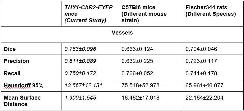
(2) Some of the chosen analysis results seem to not fully match the shown data, or the visualization of the data is hard to interpret in the current form.
We have updated the visualizations to make them more accessible and ensure close correspondence between tables and figures.
(3) Additionally, some measures seem not fully adapted to the current situation (e.g. the efficiency measure does not consider possible sources or sinks). Thus, some additional analysis work might be required to account for this.
Thank you for your comment. The efficiency metric was selected as it does not consider sources or sinks. We do agree that accounting for vessel subtypes in the analysis (thus classifying larger vessels as either suppliers/sources or drainers/sinks) would be very useful: notwithstanding, this classification is extremely laborious, as we have noted in our prior work1 . We are therefore leveraging machine learning in a parallel project to afford vessel classification by type. Notwithstanding, the source/sink analysis based on in vivo 2PFM data is confounded by the small FOV.
(4) The authors apply their method to in vivo data. However, there are some weaknesses in the design that make it hard to accept many of the conclusions and even to see that the method could yield much useful data with this type of application. Primarily, the acquisition of a large volume of tissue is very slow. In order to obtain a network of vascular activity, large volumes are imaged with high resolution. However, the volumes are scanned once every 42 seconds following stimulation. Most vascular responses to neuronal activation have come and gone in 42 seconds so each vessel segment is only being sampled at a single time point in the vascular response. So all of the data on diameter changes are impossible to compare since some vessels are sampled during the initial phase of the vascular response, some during the decay, and many probably after it has already returned to baseline. The authors attempt to overcome this by alternating the direction of the scan (from surface to deep and vice versa). But this only provides two sample points along the vascular response curve and so the problem still remains.
We thank the Reviewer for bringing up this important point. Although vessels can show relatively rapid responses to perturbation, vascular responses to photostimulation of ChannelRhodopsin-2 in neighbouring neurons are long-lasting: they do not come and go in 42 seconds. To demonstrate this point, we acquired higher temporal-resolution images of smaller volumes of tissue over 5 minutes preceding and 5 minutes following the 5-s photoactivation with the original photostimulation parameters. The imaging protocol was different in that we utilized a piezoelectric motor, a smaller field of view (512um x (80-128)um x (34-73)um), and only 3x frame averaging, resulting in a temporal resolution of 1.57-3.17 seconds per frame. This acquisition was repeated at different cortical depths in three Thy1-ChR2 mice and the vascular radii were estimated using our presented pipeline. Significantly responding vessels here were selected via an F-test of radius estimates before vs. after stimulation. LOESS fits to the time-dependent radius of significantly responding vessels are shown in Supplementary Figure 5. Vessels shorter than 20 um in length were excluded from the analysis so as to focus on vessel segments where averaging the vascular radius over many vertices was possible. A video of one of the acquisitions is shown along with the timecourses of select vessels’ calibre changes in Author response image 1. The vascular calibre changes following photostimulation persisted for several minutes, consistent with earlier observations by us and others2–5. These small-volume acquisitions demonstrated that dilations were repeatedly longer than the 42 seconds (i.e. our original temporal resolution).
Our temporal sampling was chosen to permit a large field of view acquisition while still being well within the span of the vascular response to look at larger scale vascular coordination that has not previously been studied. The pipeline readily adapts to smaller fields of view at a finer temporal sampling, though such an acquisition precludes the study of the response coordination across hundreds of vessels. While a greater number of baseline frames would help with the baseline variability estimation, maintaining animals under anesthesia during prolonged imaging is exceedingly difficult, precluding us from extending our total acquisition time.
Author response image 1.
Estimated vascular radius at each timepoint for select vessels from the imaging stack shown in the following video: https://flip.com/s/kB1eTwYzwMJE
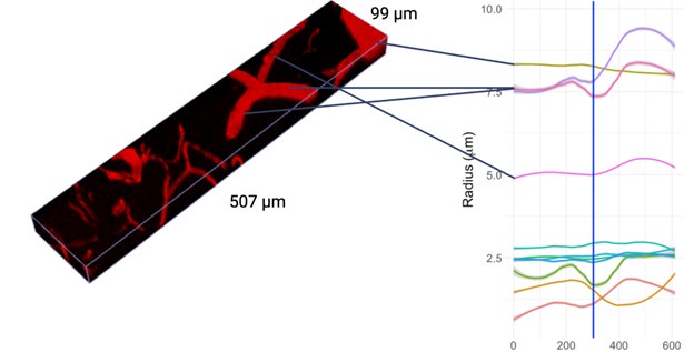
(5) A second problem is the use of optogenetic stimulation to activate the tissue. First, it has been shown that blue light itself can increase blood flow (Rungta et al 2017). The authors note the concern about temperature increases but that is not the same issue. The discussion mentions that non-transgenic mice were used to control for this with "data not shown". This is very important data given these earlier reports that have found such effects and so should be included.
We have updated the manuscript to incorporate the data on volumetric scanning in (nontransgenic) C57BL/6 mice undergoing blue light stimulation, with identical parameters as those used in Thy-ChR2 mice (Supplementary Figure 8). As before, responders were identified as vessels that following blue light stimulation showed a radius change greater than 2 standard deviations of their baseline radius standard deviation: their estimated radii changes are shown in Supplementary Figure 8. There was no statistical difference between the radii distributions of any of the photostimulation conditions and pre-photostimulation baseline.
(6) Secondly, there doesn't seem to be any monitoring of neural activity following the photo-stimulation. The authors repeatedly mention "activated" neurons and claim that vessel properties change based on distance from "activated" neurons. But I can't find anything to suggest that they know which neurons were active versus just labeled. Third, the stimulation laser is focused at a single depth plane. Since it is single-photon excitation, there is likely a large volume of activated neurons. But there is no way of knowing the spatial arrangement of neural activity and so again, including this as a factor in the analysis of vascular responses seems unjustified.
Given the high fidelity of Channel-Rhodpsin2 activation with blue light photostimulation found by us and others3, we assume that all labeled neurons within the volume of photostimulation are being activated. Depending on their respective connectivities, their postsynaptic neurons (whether or not they are labeled) may also get activated. We therefore agree with the reviewer that the spatial distribution of neuronal activation is not well defined. The manuscript has been revised to update the terminology from activated to labeled neurons and stress in the Discussion that the motivation for assessing the distance to the closest labeled neuron as one of our metrics is purely to demonstrate the possibility of linking vascular response to activations in their neighbouring neurons and including morphological metrics in the computational pipeline.
(7) The study could also benefit from more clear illustration of the quality of the model's output. It is hard to tell from static images of 3-D volumes how accurate the vessel segmentation is. Perhaps some videos going through the volume with the masks overlaid would provide some clarity. Also, a comparison to commercial vessel segmentation programs would be useful in addition to benchmarking to the ground truth manual data.
We generated a video demonstrating the deep-learning model outputs and have made the video available here: https://flip.com/s/_XBs4yVxisNs. We aimed to develop an open-source method for the research community as the vast majority of groups do not have access to commercial software for vessel segmentation.
(8) Another useful metric for the model's success would be the reproducibility of the vessel responses. Seeing such a large number of vessels showing constrictions raises some flags and so showing that the model pulled out the same response from the same vessels across multiple repetitions would make such data easier to accept.
We have generated a figure demonstrating the repeatability of the vascular responses following photostimulation in a volume and presented them next to the corresponding raw acquisitions for visual inspection (Supplementary figure 6). It is important to note that there is a significant biological variability in vessels’ responses to repeated stimulation, as described previously 3,6: a well-performing model should be able to quantify biological heterogeneity as it of itself may be of interest. Constrictions have been reported in the literature by our group and others 1,2,4,5,7, though their prevalence has not been systematically studied to date. Concerning the reproducibility of our analysis, we have demonstrated model reproducibility (as a metric of its success) on a dataset where vessels visually appeared to dilate consistently following 452 nm light stimulation: these results are now presented in Supplementary Figure 6 of the revised Manuscript. We thus observed that the model repeatedly detected the vessels - that appeared to dilate on visual inspections - as dilating. Examples of vessels constricting repeatedly were also examined and maximal intensity projections of the vessel before and after photostimulation inspected, confirming their repeated constriction (Author response image 2).
It is also worth noting that while the presence of the response (defined as change above 2 standard deviations of the radius across baseline frames) was infrequent (2107 vessels responded at least once, out of a total of 10,552 unique vessels imaged), the direction of the response was highly consistent across trials. Given twice the baseline variability as the threshold for response, of the vessels that responded more than once, 31.7% dilated on some trials while constricting on others; 41.1% dilated on each trial; and 27.2% constricted on each trial. (Note that some trials use 1.1 vs. 4.3 mW/mm2 and some have opposite scanning directions).
Author response image 2.
Sample capillaries constrictions from maximum intensity projections at repeated time points following optogenetic stimulation. Baseline (pre-stimulation) image is shown on the left and the post-stimulation image, is on the right, with the estimated radius changes listed to the left.
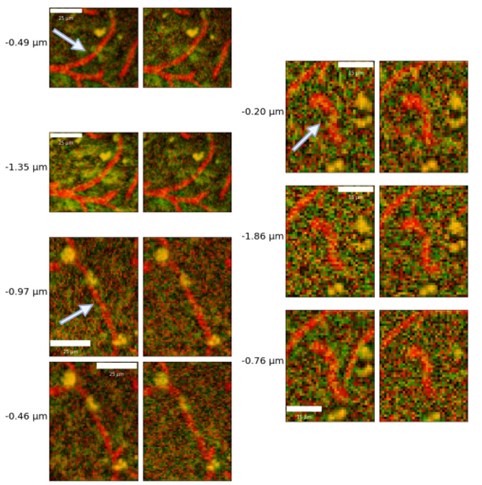
(9) A number of findings are questionable, at least in part due to these design properties. There are unrealistically large dilations and constrictions indicated. These are likely due to artifacts of the automated platform. Inspection of these results by eye would help understand what is going on.
Some of the dilations were indeed large in magnitude. We present select examples of large dilations and constrictions ranging in magnitude from 2.08 to 10.80 um for visual inspection (Author response image 3) (for reference, average, across vessel and stimuli, the magnitude of radius changes were 0.32 +/- 0.54 um). Diameter changes above 5 um were visually inspected.
Author response image 3.
Additional views of diameter change in maximum intensity projections ranging in magnitude from 2.08 um to 10.80 um.
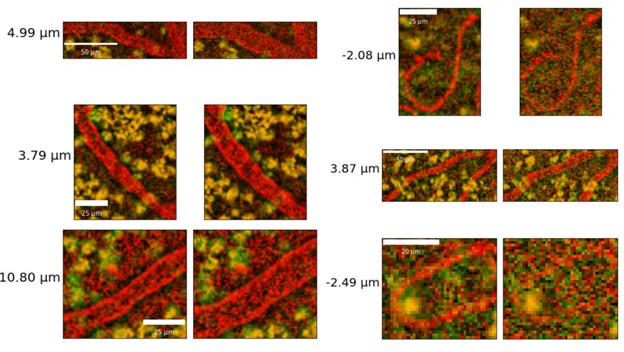
(10) In Figure 6, there doesn't seem to be much correlation between vessels with large baseline level changes and vessels with large stimulus-evoked changes. It would be expected that large arteries would have a lot of variability in both conditions and veins much less. There is also not much within-vessel consistency. For instance, the third row shows what looks like a surface vessel constricting to stimulation but a branch coming off of it dilating - this seems biologically unrealistic.
We now plot photostimulation-elicited vessel-wise radius changes vs. their corresponding baseline radius standard deviations (Author response image 4). The Pearson correlation coefficient between the baseline standard deviation and the radius change was 0.08 (p<1e-5) for 552nm 4.3 mW/mm^2 stimulation, -0.08 (p<1e-5) for 458nm 1.1 mW/mm^2 stimulation, and -0.04 (p<1e-5) for 458nm 4.3 mW/mm^2 stimulation. For non-control (i.e. blue) photostimulation conditions, the change in the radius is thus negatively correlated to the vessel’s baseline radius standard deviation: this small negative correlation indicates that there is little correlation between vessel radius change and the baseline variability in the vessel radius. Classification of vessels by type (arteries vs. veins) is needed before we can comment on differences between these vascular components. The between-vessel (i.e. between parent vessels and their daughter branches separated by branch points) consistency is explicitly evaluated by the assortativity metric, in Figure 9: vessels do somewhat tend to react similarly to their downstream branches: we observed a mean assortativity of 0.4. As for the instance of a surface vessel constricting while a downstream vessel dilates, it is important to remember that the 2PFM FOV restricts us to imaging a very small portion of the cortical microvascular network: one (among many) daughter vessels showing changes in the opposite direction to the parent vessel is not violating the conservation of mass; in addition, mural cells on adjacent branches can respond differently.
Author response image 4.
Vessel radius change elicited by photostimulation vs. baseline radius standard deviation across all vessels. The threshold level for response identification is shown as the black line.
(11) As mentioned, the large proportion of constricting capillaries is not something found in the literature. Do these happen at a certain time point following the stimulation? Did the same vessel segments show dilation at times and constriction at other times? In fact, the overall proportion of dilators and constrictors is not given. Are they spatially clustered? The assortativity result implies that there is some clustering, and the theory of blood stealing by active tissue from inactive tissue is cited. However, this theory would imply a region where virtually all vessels are dilating and another region away from the active tissue with constrictions. Was anything that dramatic seen?
The kinetics of the vascular responses are not accessible via the current imaging protocol and acquired data; however, this computational pipeline can readily be adapted to test hypotheses surrounding the temporal evolution of the vascular responses, as shown in Supplementary Figure 2 (with higher temporal-resolution data). Some vessels dilate at some time points and constrict at others as shown in Supplementary Figure 2. As listed in Table 2, 4.4% of all vessels constrict and 7.5% dilate for 452nm stimulation at 4.3 mW/mm^2. There was no obvious spatial clustering of dilators or constrictors: we expect such spatial patterns to be more common with different modes of stimulation and/or in the presence of pathology. The assortativity peaked at 0.4 (quite far from 1 where each vessel’s response exactly matches that of its neighbour).
(12) Why were nearly all vessels > 5um diameter not responding >2SD above baseline? Did they have highly variable baselines or small responses? Usually, bigger vessels respond strongly to local neural activity.
In Author response image 5, we now present the stimulation-induced radius changes vs. baseline radius variability across vessels with a radius greater than 5 um. The Pearson correlation between the radius change and the baseline radius standard deviation across time was low: r=0.05 (p=0.5) for 552nm 4.3 mW/mm^2 stimulation, r=-0.27 (p<1e-5) for 458nm 1.1 mW/mm^2 stimulation, and r=-0.31 (p<1e-5) for 458nm 4.3 mW/mm^2 stimulation. These results demonstrate that the changes following optogenetic stimulation are lower than twice the baseline standard deviation across time for most of these vessels. The pulsatility of arteries results in significant variability in their baseline radius8; in turn, literature to date suggests very limited radius changes in veins. Both of these effects could contribute to the radius response not being detected in many larger vessels.
Author response image 5.
The change in the vessel radius elicited by photostimulation vs. baseline vessel radius standard deviation in vessels with a baseline radius greater than 5 um. The threshold level for response identification is shown as the black line.
References
(1) Mester JR, Rozak MW, Dorr A, Goubran M, Sled JG, Stefanovic B. Network response of brain microvasculature to neuronal stimulation. NeuroImage. 2024;287:120512. doi:10.1016/j.neuroimage.2024.120512
(2) Alarcon-Martinez L, Villafranca-Baughman D, Quintero H, et al. Interpericyte tunnelling nanotubes regulate neurovascular coupling. Nature. 2020;kir 2.1(7823):91-95. doi:10.1038/s41586-020-2589-x
(3) Mester JR, Bazzigaluppi P, Weisspapir I, et al. In vivo neurovascular response to focused photoactivation of Channelrhodopsin-2. NeuroImage. 2019;192:135-144. doi:10.1016/j.neuroimage.2019.01.036
(4) O’Herron PJ, Hartmann DA, Xie K, Kara P, Shih AY. 3D optogenetic control of arteriole diameter in vivo. Nelson MT, Calabrese RL, Nelson MT, Devor A, Rungta R, eds. eLife. 2022;11:e72802. doi:10.7554/eLife.72802
(5) Hartmann DA, Berthiaume AA, Grant RI, et al. Brain capillary pericytes exert a substantial but slow influence on blood flow. Nat Neurosci. Published online February 18, 2021:1-13. doi:10.1038/s41593-020-00793-2
(6) Mester JR, Bazzigaluppi P, Dorr A, et al. Attenuation of tonic inhibition prevents chronic neurovascular impairments in a Thy1-ChR2 mouse model of repeated, mild traumatic brain injury. Theranostics. 2021;11(16):7685-7699. doi:10.7150/thno.60190
(7) Hall CN, Reynell C, Gesslein B, et al. Capillary pericytes regulate cerebral blood flow in health and disease. Nature. 2014;508(7494):55-60. doi:10.1038/nature13165
(8) Meng G, Zhong J, Zhang Q, et al. Ultrafast two-photon fluorescence imaging of cerebral blood circulation in the mouse brain in vivo. Proc Natl Acad Sci U S A. 2022;119(23):e2117346119. doi:10.1073/pnas.2117346119
Recommendations for the authors:
Reviewer #1 (Recommendations For The Authors):
Line 207: a superfluous '.' before the references.
This has been corrected.
Line 273 ff:
While the metrics are described in mathematical terms which is very useful, the appearing distances (d) and mathematical symbols are not. While mostly intuitively clear, precise definitions of all symbols introduced should be given to avoid ambiguities.
The description has been clarified.
This applies to all formulas appearing in the manuscript and the authors might want to check them carefully.
We have updated them wherever needed.
The mean surface distance seems not to reflect the mean MINIMAL surface distance but just the overall mean surface distance. Or a different definition of the appearing symbols is used, highlighting the need for introducing every mathematical symbol carefully.
The definitions have been updated for clarity, specifying the distinction between Hausdorff 95% distance and mean surface distance.
Line 284:
It is unclear to me why center-line detection was performed in MATLAB and not Python. Using multiple languages/software packages and in addition relying on one that is not freely available/open source makes this tool much less attractive as a real open-source tool for the community. The authors stress in the manuscript abstract that their pipeline is an open and accessible tool, the use of MATLAB defies this logic to some extent in my view.
Centerline detection for large volumetric data is available in Python, see e.g. Scipy packages as well for large data sets via ClearMap or VesselVio.
We tested the centerline detection in Python, scipy (1.9.3) and Matlab. We found that the Matlab implementation performed better due to its inclusion of a branch length parameter for the identification of terminal branches, which greatly reduced the number of false branches; the Python implementation does not include this feature (in any version) and its output had many more such “hair” artifacts. Clearmap skeletonization uses an algorithm by Palagyi & Kuba(1999) to thin segmentation masks, which does not include hair removal. Vesselvio uses a parallelized version of the scipy implementation of Lee et al. (1994) algorithm which does not do hair removal based on a terminal branch length filter; instead, Vesselvio performs a threshold-based hair removal that is frequently overly aggressive (it removes true positive vessel branches), as highlighted by the authors.
Moreover, the authors mention that robust center-line detection was critical. In my view, robust center-line extraction typically requires some additional processing of the binarized data, e.g. using a binary smoothing step. Various binary smoothers are available in the literature and as Python code.
Indeed, binary smoothing was performed: background “holes” located within the vasculature were filled; the masks were dilated (3x) and then eroded to the centreline. Scipy’s binary closing function smoothes the morphology of binary segmentation masks by dilating and then eroding the segmentation masks (as a part of the selected skeletonization algorithm).
Line 303:
'RBC' is not defined (red blood cells?)
This has been updated.
Line 398:
pPhotonsimulation -> Photostimulation
This has been corrected.
Line 400 ff: Efficiency:
I am not sure how useful the measure really is without any information about the 'sources' (i.e. arteries) and sinks (i.e. veins) as blood does not need to be moved between any two arbitrary nodes.
While blood reversals are observed, blood is typically not moved arbitrarily between two arbitrary nodes in capillary networks.
We agree with the reviewer that classifying the vessels by type is important and are currently working on deep learning-based algorithms for the classification of microvasculature into arterioles and venules for future work.
In addition, short paths between two nodes with low resistivity will potentially dominate the sum and the authors excluded vessels 10um and above. This threshold seems arbitrary.
The 10-um diameter threshold was not applied in the computation of the network metrics. The 10-um thresholding was restricted to “capillary” identification in Figure 8: the 10-um cutoff for referring to a vessel as a capillary has long been applied in the literature [1], [2], [3], [4], [5], [6], [7], [8], [9], [10], [11].
Figure 3:
It's unclear what the units are for the Mean Surface and Harsdorf Distances (pixel or um?).
The units have now been specified (um).
Figure 4:
The binarized data, and particularly the crops are difficult to interpret in black and white. It would be much more useful to present the segmentation results in a way that is interpretable (e.g. improving the rendering of the 3d information, particularly in the crops by using shadows or color codes for depth, etc).
We have updated these visualizations and shaded them based on cortical depth.
Panel C indicates that the illastik is performing badly due to changes in imagining conditions (much higher background level). As pointed out before, in my view, a reasonable pipeline should start by removing and standardizing background levels as well as dynamic ranges and possibly other artifacts before performing a more detailed analysis. This would also make the pipeline more robust against data from other microscopes etc as only a few preprocessing parameters might need to be adjusted.
I wonder whether after such a pre-processing step, UNET / UNETR would still perform in a way that was superior to ilastik, as ground truth data was generated with the aid of illastiks initially.
The Ilastik model is based on semi-automatically generated foreground labels in small batches. We had to break it up into small groups during manual labelling as larger groups were not able to run due to the computational limits of Ilastik. Ilastik is typically trained in an iterative fashion on a few patches at a time because it takes 2-3 hours per patch to train and the resulting model does not generalize on the remaining patches or out-of-distribution data - even with image pre-processing steps. On the reviewer's comment, we did try inputting normalized images into Ilastik, but this did not improve its results. UNET and UNETR inputs have been normalized for signal intensities.
Typical pre-processing/standard computer vision techniques with parameter tuning do not generalize on out-of-distribution data with different image characteristics, motivating the shift to DL-based approaches.
Figure 5:
This is a validation figure that might be better shown in an appendix or as a supplement.
Since this is a methodological paper, we think it is important to highlight the validation of the proposed method.
Line 476:
It's surprising that the number of vessel segments almost doubles when taking the union. Is the number of RBC plugs expected to be so high?
The etiology of discontinuities includes, but is not limited to, RBC plugs; we expect discontinuities to arise also from a very short pixel dwell time (0.067us) of the resonant scanning and have indeed observed apparent vessel discontinuities on resonant scanning that are not present with Galvano scanning using a pixel dwell time of 2us.
Section 4.4 / 4.5 :
The analysis in these sections provides mostly tables with numbers that are more difficult to read and hides possible interesting structures in the distribution of the various measures/quantities. For example, why is 5um a good choice to discriminate between small and large vessels, why not resolve this data more precisely via scatter plots?
Some distributions are shown in the appendix and could be moved to the main analysis.
Generally, visualizing the data and providing more detailed insights into the results would make this manuscript more interesting for the general reader.
The radius of vessel segments drops off after 5.0 um, as shown in Supplementary Figure 4A. The 10-um diameter thresholding is based on prior literature [1], [12], [13], [14], [15], [16], [17], [18], [19] and is used to segregate different vessel types in a conservative manner. The smallest capillaries are expected to have pericytes on their vessel walls whereas arteries are expected to have smooth muscle cells on their vessel walls. These differences in mural cells also may lead to differences in respective vessels’ reactivity.
The data summarized in Tables 1 and 2 are shown as scatter plots in Figures 8, Supplementary Fig 4 and Supplementary Fig 5.
Line 556:
The authors deem a certain change in radius as the relevant measure for responding vessels. They deem a vessel responding if it dilates by twice the std deviation in the radius.
Based on this measure they find that large vessels rarely respond.
However, I think this analysis might obscure some interesting effects:
(1) The standard deviation of the radius depends on the correct estimation of the center point. Given the limited spatial resolution the center point (voxel) obtained from the binarization and skeletonization might not lie in the actual center of the vessel. This effect will be stronger for larger vessels. Center point coordinates should thus be corrected to minimize the std in radius.
(2) Larger vessels will not necessarily have a perfectly circular shape, and thus the std measure is not necessarily a good measure of 'uncertainty' of estimating the actual radius.
(3) The above reasons possibly contribute to the fact that from Figure 6 it seems vessels with larger radii have higher std in general (as indicated above some more detailed visualization of the data instead of plain tables could reveal such effects better, e.g. scatter radius vs std). This higher std is making it harder to detect changes in larger vessels. However, with respect to the blood flow, the critical factor is the cross-section of the vessel that scales with the radius squared. Thus, a fixed change in radius for a vessel (say 1um) will induce a larger increase in the flow rate in larger vessels as the change in cross-section is also proportional to the radius of the vessel.
Thus, larger vessels to be deemed responders should probably have lower thresholds, thresholds should be taken on the cross-section change, or at least thresholds should not be higher for larger vessels as it is the case now using the higher std.
(1) The radius estimate does not depend on the precise placement of the center point as the radius is not being estimated by the distance from the center point to the boundary of the vessel. Instead, our strategy is to estimate the cross-sectional area (A) of the vessel by the Riemann sum of the sectors with the apex at the center point; the radius is then quoted as sqrt(A/pi) (Supplementary figure 3B). Thus, estimated vessel radius estimates in each cross-sectional plane are then averaged across the cross-sectional planes placed every ~1um along the vessel length. The uncertainty in the cross-sectional plane’s vessel radius, the uncertainty in the vessel radius (upon averaging the cross-sectional planes), and the uncertainty in the radius estimate across repeated measures of a state (i.e. across different samples of the baseline vs, post-photostimulation states) are all reported, and the last one used to define responding vessels.
To demonstrate the insensitivity to the precise placement of the vessel’s centrepoint, we have jittered the centerline in the perpendicular plane to the vessel tangent plane at each point along the vessel and then estimated the mean radius in 71 cross-sectional planes of larger vessels (mean radius > 5 um). The percent difference in the estimated radius at our selected vessel centrepoints vs. the jittered centrepoints is plotted above. The percent difference in the mean radius estimated was 0.64±3.44% with 2.45±0.30 um centerpoint jittering. (In contrast, photostimulation was estimated to elicit an average 25.4±18.1% change in the magnitude of the radius of larger vessels, i.e. those with a baseline radius >5um.)
(2) Indeed, the cross-sectional areas of either large or small vessels are not circles. Consequently, we are placing the vessel boundary, following other published work[20], at the minimum of the signal intensity gradients computed along thirty-six spokes emanating from the centrepoint (cf Figure 2H,K). The cross-sectional area of the vessel in the said cross-sectional plane is then estimated by summing the areas of the sectors flanked by neighbouring spokes. We do not make an assumption about the cross-sectional area being circular. We report radii of circles with the equivalent area as that of the cross-sectional areas merely for ease of communication (as most of the literature to date reports vessel radii, rather than vessel cross-sectional areas.)
To demonstrate the robustness of this approach, we show the sensitivity of vessel-wise radius estimate on the number of spokes used to estimate the radius in Supplementary Figure 3a. The radius estimate converges after 20 spokes have been used for estimation. Our pipeline utilizes 36 spokes and then excludes minima that lie over 2 STD away from the mean radius estimate across those 36 spokes. With 36 spokes, the vesselwise mean radius estimation was within 0.24±0.62% of the mean of radius estimates using 40-60 spokes.
(3) Across-baseline sample uncertainty in vessel radius is not dependent on baseline vessel caliber (i.e. this uncertainty is not larger in larger vessels).
Supplementary Figure 5 shows vessel radius changes for large vessels without a threshold defining responding or non-responding vessels. To explore the dependence of the outcomes on the threshold used to identify the responding vessels, we have explored an alternative strategy, whereby responding small vessels are identified as those vessels that show a post-photostimulation (vs. baseline) radius change of more than 10%. These data are now plotted in Supplementary Figure 10, for capillaries which is in agreement with Figure 8. These points are now also discussed in the Discussion section of the revised manuscript:
“Additionally, alternative definitions of responding vessels may be useful depending on the end goal of a study (e.g., this could mean selecting a threshold for the radius change based on a percentage change from the baseline level).”
Section 4.5.1
Why is the distance to the next neuron a good measure here? If two or more neurons are just a bit further away there will be twice or multiple times the 'load' while the measure would only indicate the distance to the shortest neuron. I wonder how the results change if those 'ensemble' effects are taken into account.
In this direction, looking for network-level effects with respect to the full spatial organization of the neurons would be very interesting to look at.
We agree with the review that this question is interesting; however, it is not addressable using present data: activated neuronal firing will have effects on their postsynaptic neighbors, yet we have no means of measuring the spread of activation using the current experimental model.
Figure 8
The scatter plots shown are only partly described (e.g. what's the line with error bars in C, why does it only appear for the high-intensity stimulation?).
Quadratic polynomial fit is shown only in C as the significant response was observed only for this condition, i.e. for the higher intensity blue photostimulation.
From the scatter plots as shown it is not clear to me why dilations happen on average further away. This might be a density effect not well visible in this representation. The data does not seem to show a clear relationship between neuron distance and Delta R.
Particularly in the right panel (high stimulation) there seems to be a similar number of close by neurons responding in both directions, but possibly a few more contracting at larger distances?
So, the overall effect does not seem as 'simple' as suggested in the title of section 4.5.1 in my view, but rather more cells start to contract at larger distances while there seems to be a more intricate balance nearby.
A more thorough analysis and visualization of the densities etc. might be needed to clarify this point.
The language has been revised to:
458-nm photostimulation resulted in a mix of constrictions and dilations with 44.1% of significantly responding vessels within 10 um of a labelled pyramidal neuron constricting and 55.1% dilating, while 53.3% of vessels further than 30 um constricted and 46.7% dilated. The cutoff distances from the closest labelled neuron were based on estimates of cerebral metabolic rate of oxygen consumption that showed a steep gradient in oxygen consumption with distance from arteries, CMRO2 being halved by 30 μm away
We added a probability density plot for significant constrictors and dilators to Figure 8 and Supplementary Figure 5.
Figure 8 Panel D / Section 4.5.2
This is a very interesting result in my view found in this study.
I am unclear how to interpret the effect. The authors state that dilators tend to be closer to the surface. Looking at the scatter plot (without real density information except the alpha value) it seems again the number of responders in both directions is about the same, but in deeper regions the contraction is just larger? This would be different, than how the authors interpret the data. It is unclear from the provided analysis/plots what is actually the case.
We added a probability density function plot of the constrictors and dilators, which shows a greater incidence of constrictions (vs. dilations). The text of the paper was then clarified to include the proportion of significant constrictors/ dilators closer than 10 um vs. further than 30 um away from the closest labeled neuron.
For the analyses above involving $Delta R$ I recommend also look how those results change when looking at changes in cross section instead, i.e. taking into account the actual vessel radius as well as discussed above.
It would be interesting to speculate here or in the discussion on a reason why vessels in deeper regions might need to contract more?
Unaddressed is the question if e.g. contraction in a vessel for small stimulation is predictive of contractions for larger stimulation or any other relationships?
Thank you for your comment. Given its hierarchical organization and high within-vessel response heterogeneity, we believe that the vasculature is best analyzed as a network. Our radius estimates come from averaged cross-sectional estimates allowing us to examine heterogeneity within individual vessel segments.
The discussion has been updated to include reasons as to why deeper vessels may contract more:
“As the blue light stimulation power increased, the mean depth of both constricting and dilating vessels increased, likely resulting from higher intensity light reaching ChR2-expressing neurons deeper in the tissue and exciting superficial neurons (and thus their postsynaptic neurons) to a greater level [21], [22]. The blue light would be expected to excite a lower number of neurons farther from the cortical surface at lower powers.”
Also, how consistent are contractions/dilations observed at a particular vessel etc.
To look at the consistency of a particular vessel's response to the 1.1 or 4.3 mW/mm^2 blue light photostimulation, we categorized all significant responses as constrictions or dilations, defining a responding vessel as that showing a change that is either > 2 x baseline vessel radius variability or >10% of the vessel’s mean baseline radius.
Given twice the baseline variability as the threshold for response, of the vessels that responded more than once, 31.7% dilated on some trials while constricting on others; 41.1% dilated on each trial; and 27.2% constricted on each trial. (Note that some trials use 1.1 vs. 4.3 mW/mm2 and some have opposite scanning directions).
Section 4.5.3
The results in assortativity are interesting. It would be interesting to look at how the increase in assortativity is mediated. For, example, is this in localized changes in some parts of the graph as visible in A or are there other trends? Do certain sub-graphs that systematically change their radius have certain properties (e.g. do activated neurons cluster there) or are these effects related to some hotspots that also show a coordinated change in control conditions (the assortativity seems not zero there)?
I already discussed if the efficiency measure is necessarily the best measure to use here without taking into account 'sources' and 'sinks'.
We plan to address this in future work once we have successfully trained models for the classification of vessels into arteries, veins, and capillaries. Capillaries will be classified based on their branch order from parent arteries to specify where in the network changes are occurring.
Figure 9
It's unclear to me why the Ohm symbol needs to be bold?
It is not bolded (just the font’s appearance).
Line 707:
"458-nm photostimulation caused capillaries to dilate when pyramidal neurons were close, and constrict when they were further away."
In my view, this interpretation is too simple, given the discussion above. A more detailed analysis could clarify this point.
The discussion on this point has been revised to:
458-nm photostimulation resulted in a mix of constrictions and dilations, with 44.1% of significantly responding vessels within 10 μm of a labelled pyramidal neuron constricting, and 55.1% dilating; while 53.3% of vessels further than 30 μm constricted and 46.7% dilated. The cutoff distances from the closest labelled neuron were based on estimates of cerebral metabolic rate of oxygen consumption that showed a steep gradient in oxygen consumption with distance from arteries, CMRO2 being halved by 30 μm away [23].
Line 740:
"The network efficiency here can be thought of as paralleling mean transit time, i.e., the time it takes blood to traverse the capillary network from the arteries to the veins".
The network efficiency as defined by the authors seems not to rely on artery/vein information and thus this interpretation is not fully correct in my view.
The authors might want to reconsider this measure for one that accounts for sources and sinks, if they like to interpret their results as in this line.
Yes, the efficiency described does not account for sources and sinks. It estimates the resistivity of capillaries, as a proxy for the ease of moving through the observed capillary nexus. Looking at the efficiency metric from graph theory does not require knowledge of the direction of blood flow, and can comment on the resistivity changes across capillary networks.
For future work, we are investigating methods of classifying vessels as arteries, capillaries, or veins. This type of analysis will provide more detailed information on paths between arteries and veins; it will not provide insight into large-scale network-wide modifications, as those require larger fields of view.
Line 754 Pipeline Limitations and Adaptability
I think the additional 'problem' of generating new training data for novel data sets or data from other microscopes etc should be addressed or the pipeline tested on such data sets.
Generating training data is typically the biggest time investment when adapting pipelines.
The generalization properties of the current pipeline are not discussed (e.g. performance on a different microscope / different brain area / different species etc.).
The public response to reviews has been updated with out-of-distribution data from other imaging protocols, microscopes, and species showing generalizability. These results have also been added to the paper as Supplementary Table 4, and Figure 6. The performance of our pipeline on these out-of-distribution data is now discussed in the updated Discussion section.
Line 810
Code availability should be coupled with the publication of this paper as it seems the main contribution. I don't see how the code can be made available after publication only. It should be directly available once the manuscript is published and it could help to make it available to the reviewers before that. It can be updated later of course.
The code is being made available.
Reviewer #2 (Recommendations For The Authors):
This analytical pipeline could be quite useful but it needs to be better demonstrated. If faster volumetric imaging is not possible, perhaps using it over a small volume would still demonstrate its utility at a smaller but more believable scale.
The higher temporal resolution scans (over smaller tissue volumes) have now been performed and the results of applying our pipeline to these data are summarized in Supplementary Figure 2.
Using sensory stimuli for neuronal activation might be a better idea than optogenetic stimulation. It isn't necessary but it would avoid the blue light issue.
The pipeline is readily applicable for analysis of vasoreactivity following different perturbers; however, the robustness of vessels’ response is higher with blue light photostimulation of ChR2 than with sensory stimuli [24]. Notwithstanding, an example of the vascular response to electrical stimulation of the contralateral forepaw is now included in Supplementary Figure 2.
This tool could be quite useful even without neural activity mapping. It obviously makes it even more powerful, but again, the utility could be demonstrated with just vascular data or even anatomical neuronal data without function.
We agree with both points, and have emphasized them in the revised discussion section.
Line 559 says the average capillary diameter change was 1.04 um. The next sentence and the table below all have different values so this is unclear.
The wording was updated to make this clearer.
Line 584 - should 458 be 552?
458 is correct.
Figure 1 - the schematic doesn't seem right - the 650 LPF with the notches is positioned to pass short light and reflect long wavelengths and the notch bands.
The figure has been updated to reflect this. The original layout was done for compactness.
References
(1) D. A. Hartmann, V. Coelho-Santos, and A. Y. Shih, “Pericyte Control of Blood Flow Across Microvascular Zones in the Central Nervous System,” Annu. Rev. Physiol., vol. 84, no. Volume 84, 2022, pp. 331–354, Feb. 2022, doi: 10.1146/annurev-physiol-061121-040127.
(2) J. Batista, “An adaptive gradient-based boundary detector for MRI images of the brain,” in 7th International Conference on Image Processing and its Applications, Manchester, UK: IEE, 1999, pp. 440–444. doi: 10.1049/cp:19990360.
(3) Y. Le, X. Xu, L. Zha, W. Zhao, and Y. Zhu, “Tumor boundary detection in ultrasound imagery using multi-scale generalized gradient vector flow,” J. Med. Ultrason., vol. 42, no. 1, pp. 25–38, Jan. 2015, doi: 10.1007/s10396-014-0559-3.
(4) X. Ren, “Multi-scale Improves Boundary Detection in Natural Images,” in Computer Vision – ECCV 2008, D. Forsyth, P. Torr, and A. Zisserman, Eds., Berlin, Heidelberg: Springer, 2008, pp. 533–545. doi: 10.1007/978-3-540-88690-7_40.
(5) C. Grigorescu, N. Petkov, and M. A. Westenberg, “Contour and boundary detection improved by surround suppression of texture edges,” Image Vis. Comput., vol. 22, no. 8, pp. 609–622, Aug. 2004, doi: 10.1016/j.imavis.2003.12.004.
(6) J. Tang and S. T. Acton, “Vessel Boundary Tracking for Intravital Microscopy Via Multiscale Gradient Vector Flow Snakes,” IEEE Trans. Biomed. Eng., vol. 51, no. 2, pp. 316–324, Feb. 2004, doi: 10.1109/TBME.2003.820374.
(7) J. Merkow, A. Marsden, D. Kriegman, and Z. Tu, “Dense Volume-to-Volume Vascular Boundary Detection,” in Medical Image Computing and Computer-Assisted Intervention - MICCAI 2016, S. Ourselin, L. Joskowicz, M. R. Sabuncu, G. Unal, and W. Wells, Eds., Cham: Springer International Publishing, 2016, pp. 371–379. doi: 10.1007/978-3-319-46726-9_43.
(8) F. Orujov, R. Maskeliūnas, R. Damaševičius, and W. Wei, “Fuzzy based image edge detection algorithm for blood vessel detection in retinal images,” Appl. Soft Comput., vol. 94, p. 106452, Sep. 2020, doi: 10.1016/j.asoc.2020.106452.
(9) M. E. Martinez-Perez, A. D. Hughes, S. A. Thom, A. A. Bharath, and K. H. Parker, “Segmentation of blood vessels from red-free and fluorescein retinal images,” Med. Image Anal., vol. 11, no. 1, pp. 47–61, Feb. 2007, doi: 10.1016/j.media.2006.11.004.
(10) A. M. Mendonca and A. Campilho, “Segmentation of retinal blood vessels by combining the detection of centerlines and morphological reconstruction,” IEEE Trans. Med. Imaging, vol. 25, no. 9, pp. 1200–1213, Sep. 2006, doi: 10.1109/TMI.2006.879955.
(11) A. F. Frangi, W. J. Niessen, K. L. Vincken, and M. A. Viergever, “Multiscale vessel enhancement filtering,” in Medical Image Computing and Computer-Assisted Intervention — MICCAI’98, W. M. Wells, A. Colchester, and S. Delp, Eds., Berlin, Heidelberg: Springer, 1998, pp. 130–137. doi: 10.1007/BFb0056195.
(12) K. Bisht et al., “Capillary-associated microglia regulate vascular structure and function through PANX1-P2RY12 coupling in mice,” Nat. Commun., vol. 12, no. 1, p. 5289, Sep. 2021, doi: 10.1038/s41467-021-25590-8.
(13) Y. Wu et al., “Quantitative relationship between cerebrovascular network and neuronal cell types in mice,” Cell Rep., vol. 39, no. 12, p. 110978, Jun. 2022, doi: 10.1016/j.celrep.2022.110978.
(14) T. Kirabali et al., “The amyloid-β degradation intermediate Aβ34 is pericyte-associated and reduced in brain capillaries of patients with Alzheimer’s disease,” Acta Neuropathol. Commun., vol. 7, no. 1, p. 194, Dec. 2019, doi: 10.1186/s40478-019-0846-8.
(15) X. Ren et al., “Linking cortical astrocytic neogenin deficiency to the development of Moyamoya disease–like vasculopathy,” Neurobiol. Dis., vol. 154, p. 105339, Jul. 2021, doi: 10.1016/j.nbd.2021.105339.
(16) J. Steinman, M. M. Koletar, B. Stefanovic, and J. G. Sled, “3D morphological analysis of the mouse cerebral vasculature: Comparison of in vivo and ex vivo methods,” PLOS ONE, vol. 12, no. 10, p. e0186676, Oct. 2017, doi: 10.1371/journal.pone.0186676.
(17) A.-A. Berthiaume et al., “Dynamic Remodeling of Pericytes In Vivo Maintains Capillary Coverage in the Adult Mouse Brain,” Cell Rep., vol. 22, no. 1, pp. 8–16, Jan. 2018, doi: 10.1016/j.celrep.2017.12.016.
(18) S. Katz, R. Gattegno, L. Peko, R. Zarik, Y. Hagani, and T. Ilovitsh, “Diameter-dependent assessment of microvascular leakage following ultrasound-mediated blood-brain barrier opening,” iScience, vol. 26, no. 6, p. 106965, Jun. 2023, doi: 10.1016/j.isci.2023.106965.
(19) J. Drouin-Ouellet et al., “Cerebrovascular and blood-brain barrier impairments in Huntington’s disease: Potential implications for its pathophysiology,” Ann. Neurol., vol. 78, no. 2, pp. 160–177, Aug. 2015, doi: 10.1002/ana.24406.
(20) K. P. McDowell, A.-A. Berthiaume, T. Tieu, D. A. Hartmann, and A. Y. Shih, “VasoMetrics: unbiased spatiotemporal analysis of microvascular diameter in multi-photon imaging applications,” Quant. Imaging Med. Surg., vol. 11, no. 3, pp. 969–982, Mar. 2021, doi: 10.21037/qims-20-920.
(21) E. L. Johnson et al., “Characterization of light penetration through brain tissue, for optogenetic stimulation.” bioRxiv, p. 2021.04.08.438932, Apr. 08, 2021. doi: 10.1101/2021.04.08.438932.
(22) S. I. Al-Juboori, A. Dondzillo, E. A. Stubblefield, G. Felsen, T. C. Lei, and A. Klug, “Light scattering properties vary across different regions of the adult mouse brain,” PloS One, vol. 8, no. 7, p. e67626, 2013, doi: 10.1371/journal.pone.0067626.
(23) P. Mächler et al., “Baseline oxygen consumption decreases with cortical depth,” PLOS Biol., vol. 20, no. 10, p. e3001440, Oct. 2022, doi: 10.1371/journal.pbio.3001440.
(24) J. R. Mester et al., “In vivo neurovascular response to focused photoactivation of Channelrhodopsin-2,” NeuroImage, vol. 192, pp. 135–144, May 2019, doi: 10.1016/j.neuroimage.2019.01.036.
-
-
-
Author Response
We would like to thank the reviewers for providing constructive feedback on the manuscript. To address the weaknesses identified, we are performing additional experiments and generating additional data, to be added to the updated manuscript.
(1) The utility of a pipeline depends on the generalization properties.
While the proposed pipeline seems to work for the data the authors acquired, it is unclear if this pipeline will actually generalize to novel data sets possibly recorded by a different microscope (e.g. different brand), or different imagining conditions (e.g. illumination or different imagining artifacts) or even to different brain regions or animal species, etc.
The authors provide a 'black-box' approach that might work well for their particular data sets and image acquisition settings but it is left …
Author Response
We would like to thank the reviewers for providing constructive feedback on the manuscript. To address the weaknesses identified, we are performing additional experiments and generating additional data, to be added to the updated manuscript.
(1) The utility of a pipeline depends on the generalization properties.
While the proposed pipeline seems to work for the data the authors acquired, it is unclear if this pipeline will actually generalize to novel data sets possibly recorded by a different microscope (e.g. different brand), or different imagining conditions (e.g. illumination or different imagining artifacts) or even to different brain regions or animal species, etc.
The authors provide a 'black-box' approach that might work well for their particular data sets and image acquisition settings but it is left unclear how this pipeline is actually widely applicable to other conditions as such data is not provided.
In my experience, without well-defined image pre-processing steps and without training on a wide range of image conditions pipelines typically require significant retraining, which in turn requires generating sufficient amounts of training data, partly defying the purpose of the pipeline. It is unclear from the manuscript, how well this pipeline will perform on novel data possibly recorded by a different lab or with a different microscope.
To address generalizability, we are performing several validation experiments with data from different 1) channels, 2) species (rat), and 3) microscopes, to highlight the robustness of our deep learning (DL) segmentation model to out-of-distribution data with different characteristics and acquisition protocols. We first used our model to segment three images (507x507 x&y, 250-170 um z) from three C57BL/6 mice acquired on the same two-photon fluorescent microscope following the same imaging protocol. The vasculature was labelled with the Texas Red dextran, as in the current experiment. In place of the EYFP signal from pyramidal neurons (2nd channel), gaussian noise was generated with a mean and standard deviation identical to the acquired vascular channel. A second set of two images(507x507 x&y, 300-400 um z) from two Fischer rats with Alexa680-dextran label in the plasma; these rats were imaged on the same two-photon fluorescence microscope, but with galvano scanners (instead of resonant scanners). A second channel of random Gaussian noise was also added here. Finally, an image of vasculature from a ex-vivo cleared mouse brain (1665x1205x780 um) imaged on a light sheet fluorescence microscope (Miltenyi UltraMicroscope Blaze) was also segmented with our model. Lectin-DyLight 649 was used to label the vasculature in this cohort. The Dice Score, Precision, Recall, Hausdorff 95%, and Mean surface distance will be reported for all of these additional image segmentations, upon generation of ground truth images. Finally, examples of the generated segmentation masks are presented in Author response image 1 for visual comparison. Of final note, should the segmentation results on a new data set be unsatisfactory, the methods downstream from segmentation are still applicable and the model can be further fine-tuned on other out-of-distribution data.
Author response image 1.
Examples of the deep learning model output on out of distribution data from a different mouse strain, from a different species (Fischer rat), and on a different microscope using a different imaging modality.
(2) Some of the chosen analysis results seem to not fully match the shown data, or the visualization of the data is hard to interpret in the current form.
We are updating the visualizations to make them more accessible and we will ensure matching between tables and figures.
(3) Additionally, some measures seem not fully adapted to the current situation (e.g. the efficiency measure does not consider possible sources or sinks). Thus, some additional analysis work might be required to account for this.
Thank you for your comment. The efficiency metric was selected as it does not consider sources or sinks. We do agree that accounting for vessel subtypes in the analysis (thus classifying larger vessels as either supplying or draining) would be uniquely useful: notwithstanding, it is extremely laborious. We are therefore leveraging machine learning in a parallel project to afford vessel classification by subtype. The source/sink analysis is also confounded by the small field-of-view of in situ 2PFM. Future work will investigate network remodelling across the whole brain with ex-vivo light sheet fluorescence microscopy.
(4) The authors apply their method to in vivo data. However, there are some weaknesses in the design that make it hard to accept many of the conclusions and even to see that the method could yield much useful data with this type of application. Primarily, the acquisition of a large volume of tissue is very slow. In order to obtain a network of vascular activity, large volumes are imaged with high resolution. However, the volumes are scanned once every 42 seconds following stimulation. Most vascular responses to neuronal activation have come and gone in 42 seconds so each vessel segment is only being sampled at a single time point in the vascular response. So all of the data on diameter changes are impossible to compare since some vessels are sampled during the initial phase of the vascular response, some during the decay, and many probably after it has already returned to baseline. The authors attempt to overcome this by alternating the direction of the scan (from surface to deep and vice versa). But this only provides two sample points along the vascular response curve and so the problem still remains.
We thank the Reviewer for bringing up this important point.
Although vessels can show relatively rapid responses to perturbation, vascular responses to photostimulation of ChannelRhodopsin-2 in neighbouring neurons are typically long lasting: they do not come and go in 42 seconds. To demonstrate this point, we acquired higher temporal-resolution images of smaller volumes of tissue over 5 minutes preceding and following the 5-s photoactivation with the original parameters. Imaging protocol was different in that we utilized a piezoelectric motor, smaller field of view, and only 3x frame averaging, resulting in a temporal resolution of 1.57-2.63 seconds. This acquisition was repeated at 4 different cortical depths (325 um, 250 um, 150um, and 40 um) in a single mouse.The vascular radii were estimated using our presented pipeline. Raw data and LOESS fits are shown in Author response image 2 (below). Vessels shorter than 20 um in length were excluded from the analysis. A video of one of the acquisitions is shown along with the timecourses of select vessels’ caliber changes in Author response image 3. The vascular caliber changes following photostimulation persisted for several minutes, consistent with earlier observations by us and others1–4. These higher temporal-resolution scans of smaller tissue volumes will be repeated in two more mice; we will therein assess the repeatability of individual vessel responses to repeated stimulations.
Author response image 2.
A. The vascular radii of multiple vessels were imaged at 4 different cortical depths, each within a 507 x (75-150) x (30-45)um tissue volume. Baseline scanning lasted for 5 minutes, followed by 5 seconds of blue or green light stimulation at 4.3 mW/mm2, and culminating in 5 minutes of post-stimulation scanning. B. LOESS fits of the vessel radius estimates for each vessel segment identified.
Author response image 3.
Estimated vascular radius at each timepoint for select vessels from the imaging stack shown in the following video: https://flip.com/s/kB1eTwYzwMJE
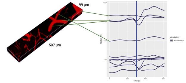
(5) A second problem is the use of optogenetic stimulation to activate the tissue. First, it has been shown that blue light itself can increase blood flow (Rungta et al 2017). The authors note the concern about temperature increases but that is not the same issue. The discussion mentions that non-transgenic mice were used to control for this with "data not shown". This is very important data given these earlier reports that have found such effects and so should be included.
We will update the manuscript to incorporate the data on volumetric scanning in nontransgenic C57BL/6 mice undergoing blue light stimulation, with identical parameters as those used in Thy-ChR2 mice. As before, responders were identified as vessels that following blue light stimulation show a radius change greater than 2 standard deviations of their baseline radius standard deviation: their estimated radii changes are shown in Author response image 4 below. There were no statistical difference between radii distributions of any of the photostimulation conditions and pre-photostimulation baseline. A comparison of this with the transgenic THY1-ChR2-EYFP mice will be included in manuscript updates.
Author response image 4.
Radius change measurements for responding vessels from the Thy1-ChR2 mice described in the manuscript (top row) vs. 4 wild-type C57BL6/J mice (bottom row). Response to photostimulation was defined as a change above twice their baseline standard deviation. 458nm light was applied at 1.1 mW/mm^2 and 4.3 mW/mm^2; while 552 nm light was applied at 4.3 mW/mm^2. No statistically significant differences were observed between the radii distributions in any condition, Wilcoxon test, Bonferroni correction.
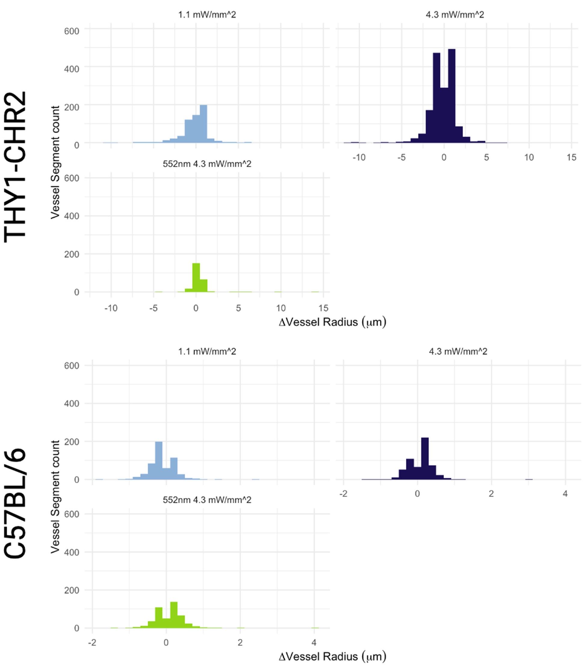
(6) Secondly, there doesn't seem to be any monitoring of neural activity following the photo-stimulation. The authors repeatedly mention "activated" neurons and claim that vessel properties change based on distance from "activated" neurons. But I can't find anything to suggest that they know which neurons were active versus just labeled. Third, the stimulation laser is focused at a single depth plane. Since it is single-photon excitation, there is likely a large volume of activated neurons. But there is no way of knowing the spatial arrangement of neural activity and so again, including this as a factor in the analysis of vascular responses seems unjustified.
Given the high fidelity of Channel-Rhodpsin2 activation with blue light, we assume that all labeled neurons within the volume of photostimulation are being activated. Depending on their respective connectivities, their postsynaptic neurons (whether or not they are labelled) are also activated. We indeed agree with the reviewer that the spatial distribution of neuronal activation is not well defined. We will revise the manuscript to update the terminology from activated to labeled neurons and stress in the Discussion that the motivation for assessing the distance to the closest labelled neuron as one of our metrics is purely to demonstrate the possibility of linking vascular response to activations in some of their neighbouring neurons and including morphological metrics in the computational pipeline. Of final note, the depth-dependence of the distance between labelled neurons and responding vessels can also readily be assessed using our computational pipeline.
(7) The study could also benefit from more clear illustration of the quality of the model's output. It is hard to tell from static images of 3-D volumes how accurate the vessel segmentation is. Perhaps some videos going through the volume with the masks overlaid would provide some clarity. Also, a comparison to commercial vessel segmentation programs would be useful in addition to benchmarking to the ground truth manual data.
We generated a video demonstrating the deep-learning model outputs and have made the video available here: https://flip.com/s/_XBs4yVxisNs Additional videos will be uploaded.
(8) Another useful metric for the model's success would be the reproducibility of the vessel responses. Seeing such a large number of vessels showing constrictions raises some flags and so showing that the model pulled out the same response from the same vessels across multiple repetitions would make such data easier to accept.
We have generated a figure demonstrating the repeatability of the vascular responses following photoactivation in a volume, and presented them next to the corresponding raw acquisitions for visual inspection. It is important to note that there is a significant biological variability in vessels’ responses to repeated stimulation, as described previously 2,5. Constrictions have been reported in the literature by our group and others 1,3,4,6,7, though their prevalence has not been systematically studied to date. Concerning the reproducibility of our analysis, we will demonstrate model reproducibility (as a metric of its success) in the updated manuscript.
Author response image 5.
Registered acquisitions of the vasculature before and after optogenetic stimulation for 5 scan pairs over 3 different stimulation conditions. The estimated radii along vessel segments are presented.
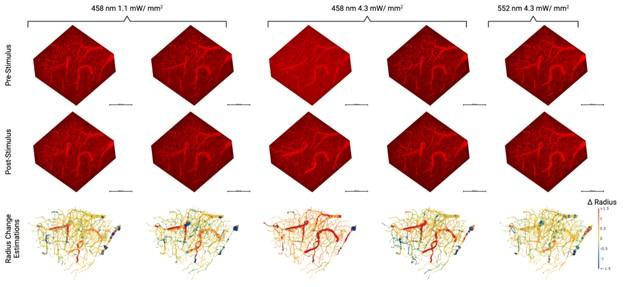
Author response image 6.
Sample capillaries constrictions from maximum intensity projections at repeated timepoints following optogenetic stimulation. Baseline (pre-stimulation) image is shown on the left and the post-stimulation image, on the right, with the estimated radius changes listed to the left.

(9) A number of findings are questionable, at least in part due to these design properties. There are unrealistically large dilations and constrictions indicated. These are likely due to artifacts of the automated platform. Inspection of these results by eye would help understand what is going on.
Some of the dilations were indeed large in magnitude. We present select examples of large dilations and constrictions ranging in magnitude from 2.08 to 10.80 um for visual inspection (for reference, average, across vessel and stimuli, magnitude of radius changes were 0.32 +/- 0.54 um). Diameter changes above 5 um were visually inspected.
Author response image 7.
Additional views of diameter changes in maximum intensity projections ranging in magnitude from 2.08 um to 10.80 um.
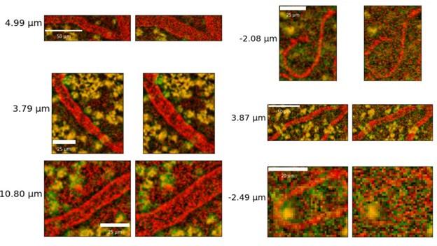
(10) In Figure 6, there doesn't seem to be much correlation between vessels with large baseline level changes and vessels with large stimulus-evoked changes. It would be expected that large arteries would have a lot of variability in both conditions and veins much less. There is also not much within-vessel consistency. For instance, the third row shows what looks like a surface vessel constricting to stimulation but a branch coming off of it dilating - this seems biologically unrealistic.
We now plot photostimulation-elicited vesselwise radius changes vs. their corresponding baseline radius standard deviations (Author response image 8 below). The Pearson correlation between the baseline standard deviation and the radius change was 0.08 (p<1e-5) for 552nm 4.3 mW/mm^2 stimulation, -0.08 (p<1e-5) for 458nm 1.1 mW/mm^2 stimulation, and -0.04 (p<1e-5) for 458nm 4.3 mW/mm^2 stimulation. For non-control (i.e. blue) photostimulation conditions, the change in the radius is thus negatively correlated to the vessel’s baseline radius standard deviation. The within-vessel consistency is explicitly evaluated in Figure 8 of the manuscript. As for the instance of a surface vessel constricting while a downstream vessel dilates, it is important to remember that the 2PFM FOV restricts us to imaging a very small portion of the cortical microvascular network (one (among many) daughter vessels showing changes in the opposite direction to the parent vessel is not violating the conservation of mass).
Author response image 8.
A plot of the vessel radius change elicited by photostimulation vs. baseline radius standard deviation.
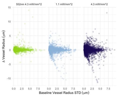
(11) As mentioned, the large proportion of constricting capillaries is not something found in the literature. Do these happen at a certain time point following the stimulation? Did the same vessel segments show dilation at times and constriction at other times? In fact, the overall proportion of dilators and constrictors is not given. Are they spatially clustered? The assortativity result implies that there is some clustering, and the theory of blood stealing by active tissue from inactive tissue is cited. However, this theory would imply a region where virtually all vessels are dilating and another region away from the active tissue with constrictions. Was anything that dramatic seen?
The kinetics of the vascular responses are not accessible via the current imaging protocol and acquired data; however, this computational pipeline can readily be adapted to test hypotheses surrounding the temporal evolution of the vascular responses, as shown in Author response image 2 (with higher temporal-resolution data). Some vessels dilate at some time points and constrict at others as shown in Author response image 2. As listed in Table 2, 4.4% of all vessels constrict and 7.5% dilate for 452nm stimulation at 4.3 mW/mm^2. There was no obvious spatial clustering of dilators or constrictors: we expect such spatial patterns to more likely result from different modes of stimulation and/or in the presence of a pathology. The assortativity peaked at 0.4 (i.e. is quite far from 1 where each vessel’s response exactly matches that of its neighbour).
(12) Why were nearly all vessels > 5um diameter not responding >2SD above baseline? Did they have highly variable baselines or small responses? Usually, bigger vessels respond strongly to local neural activity.
In Author response image 9, we now present the stimulation-induced radius changes vs. baseline radius variability across vessels with a radius greater than 5 um. The Pearson correlation between the radius change and the baseline radius standard deviation was 0.04 (p=0.5) for 552nm 4.3 mW/mm^2 stimulation, -0.26 (p<1e-5) for 458nm 1.1 mW/mm^2 stimulation, and -0.24 (p<1e-5) for 458nm 4.3 mW/mm^2 stimulation. We will incorporate an additional analysis to address this issue by identifying responding vessels as those showing supra-threshold percent change in their radius (instead of SD).
Author response image 9.
A plot of the vessel radius change elicited by photostimulation vs. baseline radius standard deviation in vessels with a baseline radius greater than 5 um.
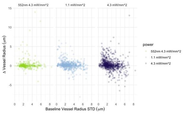
References
(1) Alarcon-Martinez L, Villafranca-Baughman D, Quintero H, et al. Interpericyte tunnelling nanotubes regulate neurovascular coupling. Nature. 2020;kir 2.1(7823):91-95. doi:10.1038/s41586-020-2589-x
(2) Mester JR, Bazzigaluppi P, Weisspapir I, et al. In vivo neurovascular response to focused photoactivation of Channelrhodopsin-2. NeuroImage. 2019;192:135-144. doi:10.1016/j.neuroimage.2019.01.036
(3) O’Herron PJ, Hartmann DA, Xie K, Kara P, Shih AY. 3D optogenetic control of arteriole diameter in vivo. Nelson MT, Calabrese RL, Nelson MT, Devor A, Rungta R, eds. eLife. 2022;11:e72802. doi:10.7554/eLife.72802
(4) Hartmann DA, Berthiaume AA, Grant RI, et al. Brain capillary pericytes exert a substantial but slow influence on blood flow. Nat Neurosci. Published online February 18, 2021:1-13. doi:10.1038/s41593-020-00793-2
(5) Mester JR, Bazzigaluppi P, Dorr A, et al. Attenuation of tonic inhibition prevents chronic neurovascular impairments in a Thy1-ChR2 mouse model of repeated, mild traumatic brain injury. Theranostics. 2021;11(16):7685-7699. doi:10.7150/thno.60190
(6) Mester JR, Rozak MW, Dorr A, Goubran M, Sled JG, Stefanovic B. Network response of brain microvasculature to neuronal stimulation. NeuroImage. 2024;287:120512. doi:10.1016/j.neuroimage.2024.120512
(7) Hall CN, Reynell C, Gesslein B, et al. Capillary pericytes regulate cerebral blood flow in health and disease. Nature. 2014;508(7494):55-60. doi:10.1038/nature13165
-
eLife assessment
This valuable work describes a highly complex automated algorithm for analyzing vascular imaging data from two-photon microscopy. This tool has the potential to fill gaps in knowledge of hemodynamic activity across a regional network. The underlying methods and results are still incomplete; the biological application provided has several problems that make many of the scientific claims in the paper questionable and the generalizability of the pipeline needs to be further addressed. We believe these concerns could be addressed.
-
Reviewer #1 (Public Review):
Summary:
In this manuscript, the authors describe a new pipeline to measure changes in vasculature diameter upon opt-genetic stimulation of neurons.
The work is interesting and the topic is quite relevant to better understand the hemodynamic response on the graph/network level.
Strengths:
The manuscript provides a pipeline that allows for the detection of changes in the vessel diameter as well as simultaneously allowing for the location of the neurons driven by stimulation.
The resulting data could provide interesting insights into the graph-level mechanisms of regulating activity-dependent blood flow.
The interesting findings include that vessel radius changes depend on depth from the cortical surface and that dilations on average happen closer to the activated neurons.
Weaknesses:
The utility of a pipeline …
Reviewer #1 (Public Review):
Summary:
In this manuscript, the authors describe a new pipeline to measure changes in vasculature diameter upon opt-genetic stimulation of neurons.
The work is interesting and the topic is quite relevant to better understand the hemodynamic response on the graph/network level.
Strengths:
The manuscript provides a pipeline that allows for the detection of changes in the vessel diameter as well as simultaneously allowing for the location of the neurons driven by stimulation.
The resulting data could provide interesting insights into the graph-level mechanisms of regulating activity-dependent blood flow.
The interesting findings include that vessel radius changes depend on depth from the cortical surface and that dilations on average happen closer to the activated neurons.
Weaknesses:
The utility of a pipeline depends on the generalization properties.
While the proposed pipeline seems to work for the data the authors acquired, it is unclear if this pipeline will actually generalize to novel data sets possibly recorded by a different microscope (e.g. different brand), or different imagining conditions (e.g. illumination or different imagining artifacts) or even to different brain regions or animal species, etc.
The authors provide a 'black-box' approach that might work well for their particular data sets and image acquisition settings but it is left unclear how this pipeline is actually widely applicable to other conditions as such data is not provided.
In my experience, without well-defined image pre-processing steps and without training on a wide range of image conditions pipelines typically require significant retraining, which in turn requires generating sufficient amounts of training data, partly defying the purpose of the pipeline.
It is unclear from the manuscript, how well this pipeline will perform on novel data possibly recorded by a different lab or with a different microscope.
Analysis
Some of the chosen analysis results seem to not fully match the shown data, or the visualization of the data is hard to interpret in the current form. Additionally, some measures seem not fully adapted to the current situation (e.g. the efficiency measure does not consider possible sources or sinks). Thus, some additional analysis work might be required to account for this.
-
Reviewer #2 (Public Review):
Summary:
The authors develop a highly detailed pipeline to analyze hemodynamic signals from in vivo two-photon fluorescence microscopy. This includes motion correction, segmentation of the vascular network, diameter measurements across time, mapping neuronal position relative to the vascular network, and analyzing vascular network properties (interactions between different vascular segments). For the segmentation, the authors use a Convolution Neural Network to identify vessel (or neural) and background pixels and train it using ground truth images based on semi-automated mapping followed by human correction/annotation. Considerable processing was done on the segmented images to improve accuracy, extract vessel center lines, and compute frame-by-frame diameters. The model was tested with artificial diameter …
Reviewer #2 (Public Review):
Summary:
The authors develop a highly detailed pipeline to analyze hemodynamic signals from in vivo two-photon fluorescence microscopy. This includes motion correction, segmentation of the vascular network, diameter measurements across time, mapping neuronal position relative to the vascular network, and analyzing vascular network properties (interactions between different vascular segments). For the segmentation, the authors use a Convolution Neural Network to identify vessel (or neural) and background pixels and train it using ground truth images based on semi-automated mapping followed by human correction/annotation. Considerable processing was done on the segmented images to improve accuracy, extract vessel center lines, and compute frame-by-frame diameters. The model was tested with artificial diameter increases and Gaussian noise and proved robust to these manipulations.
Network-level properties include Assortativity - a measure of how similar a vessel's response is to nearby vessels - and Efficiency - the ease of flow through the network (essentially, the combined resistance of a path based on diameter and vessel length between two points).
Strengths:
This is a very powerful tool for cerebral vascular biologists as many of these tasks are labor intensive, prone to subjectivity, and often not performed due to the complexity of collecting and managing volumes of vascular signals. Modelling is not my specialty so I cannot speak too specifically, but the model appears to be well-designed and robust to perturbations. It has many clever features for processing the data.
The authors rightly point out that there is a real lack in the field of knowledge of vascular network activity at single-vessel resolution. Network anatomy has been studied, but hemodynamics are typically studied either with coarse resolution or in only one or a few vessels at a time. This pipeline has the potential to change that.
Weaknesses:
The authors apply their method to in vivo data. However, there are some weaknesses in the design that make it hard to accept many of the conclusions and even to see that the method could yield much useful data with this type of application. Primarily, the acquisition of a large volume of tissue is very slow. In order to obtain a network of vascular activity, large volumes are imaged with high resolution. However, the volumes are scanned once every 42 seconds following stimulation. Most vascular responses to neuronal activation have come and gone in 42 seconds so each vessel segment is only being sampled at a single time point in the vascular response. So all of the data on diameter changes are impossible to compare since some vessels are sampled during the initial phase of the vascular response, some during the decay, and many probably after it has already returned to baseline. The authors attempt to overcome this by alternating the direction of the scan (from surface to deep and vice versa). But this only provides two sample points along the vascular response curve and so the problem still remains.
A second problem is the use of optogenetic stimulation to activate the tissue. First, it has been shown that blue light itself can increase blood flow (Rungta et al 2017). The authors note the concern about temperature increases but that is not the same issue. The discussion mentions that non-transgenic mice were used to control for this with "data not shown". This is very important data given these earlier reports that have found such effects and so should be included. Secondly, there doesn't seem to be any monitoring of neural activity following the photo-stimulation. The authors repeatedly mention "activated" neurons and claim that vessel properties change based on distance from "activated" neurons. But I can't find anything to suggest that they know which neurons were active versus just labeled. Third, the stimulation laser is focused at a single depth plane. Since it is single-photon excitation, there is likely a large volume of activated neurons. But there is no way of knowing the spatial arrangement of neural activity and so again, including this as a factor in the analysis of vascular responses seems unjustified.
The study could also benefit from more clear illustration of the quality of the model's output. It is hard to tell from static images of 3-D volumes how accurate the vessel segmentation is. Perhaps some videos going through the volume with the masks overlaid would provide some clarity. Also, a comparison to commercial vessel segmentation programs would be useful in addition to benchmarking to the ground truth manual data.
Another useful metric for the model's success would be the reproducibility of the vessel responses. Seeing such a large number of vessels showing constrictions raises some flags and so showing that the model pulled out the same response from the same vessels across multiple repetitions would make such data easier to accept.
A number of findings are questionable, at least in part due to these design properties.
There are unrealistically large dilations and constrictions indicated. These are likely due to artifacts of the automated platform. Inspection of these results by eye would help understand what is going on.
In Figure 6, there doesn't seem to be much correlation between vessels with large baseline level changes and vessels with large stimulus-evoked changes. It would be expected that large arteries would have a lot of variability in both conditions and veins much less. There is also not much within-vessel consistency. For instance, the third row shows what looks like a surface vessel constricting to stimulation but a branch coming off of it dilating - this seems biologically unrealistic.
As mentioned, the large proportion of constricting capillaries is not something found in the literature. Do these happen at a certain time point following the stimulation? Did the same vessel segments show dilation at times and constriction at other times? In fact, the overall proportion of dilators and constrictors is not given. Are they spatially clustered? The assortativity result implies that there is some clustering, and the theory of blood stealing by active tissue from inactive tissue is cited. However, this theory would imply a region where virtually all vessels are dilating and another region away from the active tissue with constrictions. Was anything that dramatic seen?
As mentioned, the claims about distance to active neurons are not meaningful if there is no measure of which neurons were active and which weren't. But even still, the claim is overly strong as the average distance to the nearest neuron for dilators was ~17 microns and for constrictors it was ~22 microns - about a half a neuronal soma difference.
The distance to the nearest neuron likely will depend on depth as well - neurons are quite sparse superficially and very dense in layer 4. The capillary network varies much less (see Blinder et al 2016 Nature Neuroscience). So the distance of a neuron to the nearest capillary may not vary much with depth, but the distance from the capillary to the nearest neuron might vary quite a lot.
Why were nearly all vessels > 5um diameter not responding >2SD above baseline? Did they have highly variable baselines or small responses? Usually, bigger vessels respond strongly to local neural activity. -
