Distinct cortical encoding of acoustic and electrical cochlear stimulation
Curation statements for this article:-
Curated by eLife

eLife Assessment
This valuable study compares auditory cortex responses to sounds and cochlear implant stimulation measured with surface electrode grids in rats. Beyond the reduced frequency resolution of cochlear implants observed previously, this study suggests key discrepancies between neuronal representations of cochlear stimulations and natural sounds. The evidence for this result is solid but could be strengthened with a clarification of the methodology and an adaptation of the claim to the actual precision of the measurements. This study is of interest to researchers in the auditory neuroscience field and clinicians implementing treatments with cochlear implants.
This article has been Reviewed by the following groups
Discuss this preprint
Start a discussion What are Sciety discussions?Listed in
- Evaluated articles (eLife)
Abstract
Cochlear implants are neuroprosthetic devices that restore hearing and speech comprehension to profoundly deaf humans, and represent an exemplar application of biomedical engineering and research to clinical conditions. However, the utility of these devices in many subjects is limited, largely due to lack of information about how neural circuits respond to implant stimulation. Recently we showed that deafened rats can use cochlear implants to recognize sounds, and that this training refined the responses of single neurons in the primary auditory cortex. Here we asked how local populations of cortical neurons represent acute implant stimuli, using electrode arrays we developed for cortical surface recordings for micro-electrocorticography (µECoG), a form of intracranial electroencephalography (iEEG). We found that there was a limited tonotopic organization across recording sites, relative to a clearer tonotopic spatial representation in normal-hearing rats. Singletrial iEEG responses to acoustic inputs were more reliable than responses to cochlear implant stimulation, although stimulus identity could be successfully decoded in both cases. However, the spatiotemporal response profiles to acoustic vs cochlear implant stimulation were substantially different. Decoders trained on acoustic responses showed essentially zero information transfer when tested on electrical stimulation responses in the same animals after deafening and cochlear implant stimulation. Thus while acute cochlear implant stimulation might activate the auditory cortex in a cochleotopic manner, the dynamics of network activity are quite distinct, suggesting that pitch percepts from acoustic and electrical stimulation are fundamentally different.
Article activity feed
-

-
-

eLife Assessment
This valuable study compares auditory cortex responses to sounds and cochlear implant stimulation measured with surface electrode grids in rats. Beyond the reduced frequency resolution of cochlear implants observed previously, this study suggests key discrepancies between neuronal representations of cochlear stimulations and natural sounds. The evidence for this result is solid but could be strengthened with a clarification of the methodology and an adaptation of the claim to the actual precision of the measurements. This study is of interest to researchers in the auditory neuroscience field and clinicians implementing treatments with cochlear implants.
-
Reviewer #1 (Public review):
Summary
This manuscript addresses an important question in auditory neuroscience and neuroprosthetics: whether cortical responses to cochlear implant stimulation resemble those evoked by natural acoustic stimulation, or whether electrical stimulation engages a distinct cortical representation. The authors use high-density intracranial EEG recordings in rats to compare responses to pure tones in normal-hearing animals with responses to single-channel cochlear implant stimulation in deafened animals. They combine analyses of event-related potentials, high-gamma activity, trial-by-trial variability, PCA/TCA-based dimensionality reduction, and decoder-based measures of stimulus information.
Strengths
A major strength of the study is the question it addresses. Understanding how electrical cochlear stimulation is …
Reviewer #1 (Public review):
Summary
This manuscript addresses an important question in auditory neuroscience and neuroprosthetics: whether cortical responses to cochlear implant stimulation resemble those evoked by natural acoustic stimulation, or whether electrical stimulation engages a distinct cortical representation. The authors use high-density intracranial EEG recordings in rats to compare responses to pure tones in normal-hearing animals with responses to single-channel cochlear implant stimulation in deafened animals. They combine analyses of event-related potentials, high-gamma activity, trial-by-trial variability, PCA/TCA-based dimensionality reduction, and decoder-based measures of stimulus information.
Strengths
A major strength of the study is the question it addresses. Understanding how electrical cochlear stimulation is represented centrally is highly relevant for cochlear implant design, fitting strategies, and rehabilitation. The comparison between acoustic and electrical stimulation, including within-animal comparisons in a subset of cases, is valuable because it directly addresses whether implant-evoked activity can be interpreted within the framework of normal acoustic tonotopy.
The methodological approach is also a strength. Dense cortical surface recordings provide simultaneous access to spatial and temporal features of auditory cortical responses. The combination of PCA, TCA, and decoder analyses gives complementary views of the data, and the information-transfer analysis provides an interesting way to ask whether representations learned from acoustic stimulation generalize to electrical stimulation.
Weaknesses:
The main weakness is that the evidence for spatial organization remains difficult to interpret. In Figure 2, the authors argue that both tone-evoked and cochlear implant-evoked responses are spatially organized, but the slope analyses are not significant for the cochlear implant condition. The revised vector-strength analysis supports the presence of non-random spatial structure, but this is not the same as demonstrating a clear graded cochleotopic organization. The manuscript would be strongest if it consistently distinguished between non-random spatial structure, coarse topography, and true graded tonotopy or cochleotopy.
A related issue is that some figure titles and interpretive statements still appear stronger than the data justify. For example, the TCA results in Figure 7 are described as revealing topographically organized latent spatial factors, but the statistical support appears strongest for normal-hearing high-gamma responses, with weaker or non-significant results in other conditions. These data remain interesting, but they would be better framed as evidence for weak or coarse spatial structure rather than robust topographic organization across all modalities.
The decoder analyses are improved, especially with the added tone-to-tone control. This control supports the conclusion that poor acoustic-to-CI transfer is not simply a failure of the TCA/LDA pipeline. However, the analysis remains model-dependent, and the absolute information transfer values are low. It would be helpful either to include an analogous analysis using raw ERP/high-gamma features or to explain more explicitly why the TCA-based approach is the appropriate primary test. The data support poor generalization between acoustic and implant-evoked cortical responses, but claims about perceptual qualities should remain speculative because perception is not directly measured in these experiments.
Finally, although methodological reporting is much improved, some verification remains indirect. The authors provide useful implantation criteria and cite prior validation of their deafening approach, but the manuscript would be clearer if it explicitly distinguished between validation performed in the present animals and validation based on previous cohorts. This distinction is important because surgical variability, implantation efficacy, and deafening completeness can influence the interpretation of cochlear implant experiments.
Comments on revised version.
The revised manuscript is considerably improved. The authors have clarified several methodological details, added a statistical framework that better accommodates both paired and unpaired animals, provided a clearer account of animal cohorts, added peripheral ECAP/forward-masking data to support the cochlear specificity of implant stimulation, and included a useful positive control for the cross-modal decoder analysis. These additions make the manuscript stronger and help readers interpret the main findings more confidently.
The results support the conclusion that acoustic and cochlear implant stimulation evoke cortical responses with different properties. In particular, acoustic responses support better single-trial stimulus decoding than cochlear implant responses, and decoders trained on acoustic responses transfer poorly to implant-evoked responses. The evidence for spatial organization is more nuanced. The cochlear implant condition shows evidence of non-random spatial structure, but not a clear graded cochleotopic map. The normal-hearing condition is also less visually clear than might be expected from prior tonotopy studies, although the added analyses and comparisons to previous work help contextualize this result. Overall, the study makes a valuable contribution, provided that the claims about spatial organization and perceptual interpretation remain appropriately cautious.
The revision addresses several important concerns from the original version. The use of mixed-effects models better matches the partially paired experimental design. The expanded Methods improve reproducibility. The new cohort schematic helps clarify which animals contributed to behavioral and neural datasets. The ECAP forward-masking measurements add useful peripheral validation, and the within-modality decoder control strengthens the interpretation of the poor cross-modal transfer result. Together, these changes substantially improve the manuscript.
The work is likely to be of interest to auditory neuroscientists, cochlear implant researchers, and neuroengineers. Even where some conclusions require cautious wording, the dataset and analytical framework may be useful for future studies aiming to relate cortical responses to implant programming, perceptual learning, or closed-loop neuroprosthetic approaches.
Overall, the revised manuscript is stronger and addresses an important problem with useful methods and analyses. The results most convincingly show that acoustic responses support better single-trial decoding than acute cochlear implant responses, and that acoustic-trained decoders generalize poorly to implant-evoked activity. The evidence for robust spatial organization, especially in the cochlear implant condition, is more limited and should be presented with appropriate caution.
-
Reviewer #2 (Public review):
Summary:
This article reports measurements of iEEG signals on the rat auditory cortex during cochlear implant or sound stimulation in separate groups of rats. The observations indicate some spatial organization of cochlear implant stimuli, but that is very different from cochlear implants.
Strengths:
The study includes interesting analyses of the sound and cochlear implant representation structure based on decoders.
Weaknesses:
The observation that responses to cochlear implant stimulation (stimulation) is spatially organized is not new (e.g. Adenis et al. 2024)
The claim that spatial and temporal dimensions contribute information about the sound is also not new there is a large literature on this topic.
The analyses supporting the claim that there is a mismatch between cochlear implant and sound …
Reviewer #2 (Public review):
Summary:
This article reports measurements of iEEG signals on the rat auditory cortex during cochlear implant or sound stimulation in separate groups of rats. The observations indicate some spatial organization of cochlear implant stimuli, but that is very different from cochlear implants.
Strengths:
The study includes interesting analyses of the sound and cochlear implant representation structure based on decoders.
Weaknesses:
The observation that responses to cochlear implant stimulation (stimulation) is spatially organized is not new (e.g. Adenis et al. 2024)
The claim that spatial and temporal dimensions contribute information about the sound is also not new there is a large literature on this topic.
The analyses supporting the claim that there is a mismatch between cochlear implant and sound representation are still unclear, particularly in Fig. 8.
-
Reviewer #3 (Public review):
Summary:
Through micro-electroencephalography, Hight and colleagues studied how the auditory cortex in its ensemble respond to cochlear implant stimulation compared to the classic pure tones. Taking advantage of a double implanted rat model (Micro-ECoG and Cochlear Implant), they tracked and analyzed changes happening in the temporal and spatial aspects of the cortical evoked responses in both normal hearing and cochlear-implanted animals. After establishing that single trial responses were sufficient to encode the stimuli properties, the authors then explored several decoder architectures to study the cortex ability to encode each stimuli modality in a similar or different manner. They conclude that a) intracranial EEG evoked responses can be accurately recorded and did not differed between normal hearing …
Reviewer #3 (Public review):
Summary:
Through micro-electroencephalography, Hight and colleagues studied how the auditory cortex in its ensemble respond to cochlear implant stimulation compared to the classic pure tones. Taking advantage of a double implanted rat model (Micro-ECoG and Cochlear Implant), they tracked and analyzed changes happening in the temporal and spatial aspects of the cortical evoked responses in both normal hearing and cochlear-implanted animals. After establishing that single trial responses were sufficient to encode the stimuli properties, the authors then explored several decoder architectures to study the cortex ability to encode each stimuli modality in a similar or different manner. They conclude that a) intracranial EEG evoked responses can be accurately recorded and did not differed between normal hearing and cochlear-implanted rats; b) Although coarsely spatially organized, CI-evoked responses had higher trial-by-trial variability than pure tones; c) Stimulus identity is independently represented by temporal and spatial aspect of cortical representations and can be accurately decoded by various means from single trials; d) and that Pure tones trained decoder can't decode CI-stimulus identity accurately.
Strength:
The model combining micro-eCoG and cochlear implantation and the methodology to extract both the Event Related Potentials (ERPs) and High-Gammas (HGs) is very well designed and appropriately analyzed. Likewise, the PCA-LDA and TCA-LDA are powerful tools that take full advantage of the information provided by the cortical ensembles.
The overall structure of the paper, with a paced and exhaustive progress through each step and evolution of the decoder is very appreciable and easy to follow. The exploration of single trial encoding and stimulus identity through temporal and spatial domains is providing new avenues to characterize the cortical responses CI stimulations and their central representation. The fact that single trials suffice to decode the stimulus identity regardless of their modality is of great interest and noteworthy. Although the authors confirm that iEEG remains difficult to transpose in clinic, the insights provided by the study confirm the potential benefit of using central decoders to help in clinic settings.
Weakness:
The conclusion of the paper, especially the concept of distinct cortical encoding for each modality, is unfortunately partially supported by the results as the authors ignored fundamental limitations of CI related stimulation.
First, the authors stimulated in a Monopolar mode which, albeit being clinically relevant, notoriously generates a high current spread in rodent models. Comparing the averaged BF maps for iEEG (Fig-2A, C), BFs ranged from 4 to 16kHz with a predominance of 4kHz BFs. The lack of BFs at higher frequencies might reveal a potential location mismatch between the frequency range sampled at the level of the cortex (low to medium frequencies) and the frequency range covered by the CI inserted mostly in the first turn-and-a-half of the cochlea (high to medium frequencies). Looking at Fig-2F (and to some extend 2A) most of CI electrodes elicited responses around the 4kHz regions and averaged maps show a predominance of CI-3-4 across cortex (Fig-2C, H and Sup Fig. 3) from areas with 4kHz BF to areas with 16kHz BF. It is doubtful that CI-3-4 are located near the 4kHz region based on Müller's work (1991) on the frequency representation in the rat cochlea. Moreover, Supplemental figure 3 shows that only a couple of CI electrodes are predominately represented at the level of the cortex. Thus, it seems possible that current spread ended stimulating indistinctly higher turns of the cochlea or even the modiolus in a non-specific manner, greatly reducing (or smearing) the place-coding/frequency resolution of each electrode, which in turn could explain the coarse topographic (or coarsely tonotopic according to the manuscript) organization of the cortical responses.
Second, although the authors acknowledge that post-lingual CI users always have an adaptation period, their conclusion is based on measurements that are relatively "early" in the CI-use timeline so to speak since iEEG were collected a) acutely right after mono-aural implantation and stimulation, b) under anesthesia, c) using unmodulated pulse train fixed at 900pps regardless of the electrode used and thus lacking any temporal information shifts in relationship to electrode cochleotopic placement. Basically, all CI electrodes had the same rate whereas you would expect basal CI electrodes to be amplitude modulated at higher frequencies than apical electrodes.
As much as the reviewer likes the overall approach with the use of PCA-LDA and TCA, and agrees that information transfer seems inexistant at time of measurement, authors should be more careful in their strong conclusion that two distinct encoding exist. The non-overlapping between sound and electric stimulation representations might exist only transiently and this should be acknowledged a bit more in the discussion. Without repetition of iEEG measurement at later period with chronic use of the CI, it is not possible to definitively claim that two distinct, non-overlapping coding co-exist at all times.
Nevertheless, the reviewer wants to reiterate that the study proposed by Hight et al. is well constructed, relevant to the field and that the overall proposal of improving patient performances and help their adaptation in the first months of CI use by studying central responses should be pursued as it might help establish new guidelines or create new clinical tools.
-
Author response:
The following is the authors’ response to the original reviews
Summary of revision for all referees:
We thank referees for their constructive comments. To address their concerns, we now performed additional statistical analyses integrating both paired and unpaired data, performed positive controls for comparisons between NH- and CI- evoked iEEG measurements, developed tools for measuring and collected new experimental data on forward masking ECAP measurements in CI implanted rats (N=3), and reworked both manuscript text and figures to improve clarity. These most significant changes are summarized here, and a complete list of responses to reviewers and corresponding changes will follow.
Summary of major changes to revised manuscript:
(1) Statistical treatment of paired vs unpaired recordings using mixed-effects models …
Author response:
The following is the authors’ response to the original reviews
Summary of revision for all referees:
We thank referees for their constructive comments. To address their concerns, we now performed additional statistical analyses integrating both paired and unpaired data, performed positive controls for comparisons between NH- and CI- evoked iEEG measurements, developed tools for measuring and collected new experimental data on forward masking ECAP measurements in CI implanted rats (N=3), and reworked both manuscript text and figures to improve clarity. These most significant changes are summarized here, and a complete list of responses to reviewers and corresponding changes will follow.
Summary of major changes to revised manuscript:
(1) Statistical treatment of paired vs unpaired recordings using mixed-effects models (updates to all manuscript figures that compare NH vs CI); this largely confirmed the results reported in our original submission.
(2) New analysis, controlling for information-theoretic cross-modality comparison (i.e., training with tone- and testing with cochlear implant-evoked iEEG measures, Fig. 8).
(3) Clarification of methods (Supplemental Fig. 2 & manuscript text)
(4) Additional experiments testing peripheral tuning of our 8-channel CI rodent model via forward masking ECAP measures across 3 animals (N=3, Supplemental Fig. 1)
(5) Detailed response addressing robustness of tonotopy in NH and CI animals
Public Reviews:
Reviewer #1 (Public Review):
Strengths:
The study poses a timely, clinically relevant question with clear implications for CI strategy. The analytical toolkit is appropriate: µECoG captures mesoscale patterns; TCA offers a transparent separation of spatial and temporal structure; and mutual-information decoding provides an interpretable measure of single-trial discriminability. Within-subject recordings in a subset of animals, in principle, help isolate modality effects from inter-animal variability. Where analyses are most direct, the acoustic condition yields higher single-trial decoding accuracy, which is a meaningful and clearly presented result.
We appreciate the comments on the strengths of our analytic approaches.
Weaknesses:
Parts of the statistical treatment do not match the data structure: some comparisons mix paired and unpaired animals but are analysed as fully paired, raising concerns about misestimated uncertainty.
Please see our response to specific comment #2 above. In short, we agree with this critique of our original analyses, and in our revised manuscript we re-analyzed all NH vs. CI comparisons using linear mixed effects models that incorporate both paired and unpaired observations within a single framework. This allows us to include all animals, account for within-animal dependence for paired experiments (normal hearing and cochlear implant data from the same animal when available), and to align the statistical tests with the data shown in the figures. In almost every case, the mixed effects models confirm our original conclusions. Two comparisons that were previously nonsignificant now reach criterion for statistical significance (Fig. 2E, p=0.048 and Fig. 6F, p=0.027). We updated the manuscript to report these values and to clarify the use of mixed effects modeling in the methods under the section titled, “Linear mixed effects modeling.”
Methodological reporting is incomplete in places; essential parameters for both acoustic and electrical stimulation, as well as objective verification of implantation and deafening, are not described with sufficient detail to support confident interpretation or replication.
Please see our response to comment #5 below. We have revised our manuscript to now include this information in the methods.
Figure-level clarity also undermines the message. In Figure 2, non-significant slopes for CI, repeated identification of a single "best channel," mismatched axes, and unclear distinctions between example and averaged panels make the assertion of spatial organisation unconvincing; importantly, the normal-hearing panels also do not display tonotopy as clearly as expected, which weakens the key contrast the paper seeks to establish.
This is an important point, thanks- please see responses to comment #1 above. We note that conventional tonotopic maps in auditory cortex are characteristic frequency maps, i.e., maps of topographic organization for responses to lowest-threshold stimuli (often presented around 20-50 dB SPL). Our maps were constructed from stimuli presented at 70 dB SPL, thus blunting crisp tonotopy to some degree. Furthermore, we quantified spatial organization using a previously published method from the Polley lab (Romero & Hight et al. 2020), in which local tonotopic gradient vectors (magnitude and direction) were computed from GCaMP responses at each pixel and projected onto a unit circle. Mean vector strength across all pixels was then compared to a shuffled distribution as a measure of tonotopic organization. We applied the same procedure to our iEEG best-frequency and best-channel maps. Both map types yielded mean vector strengths that were substantially larger than those derived from shuffled maps (p < 10-10), indicating that our maps have a consistent tonotopic (for BFs) or cochleotopic (for CI channels) organization that is highly unlikely to arise by chance. This is now included in our revised manuscript.
Finally, the decoding claims would be strengthened by simple internal controls, such as within modality train/test splits and decoding on raw ERP/high-gamma features to demonstrate that poor cross-modal transfer reflects genuine differences in the underlying responses rather than limitations of the modelling pipeline.
Please see our response to comment #12 below. In short, we have now included this analysis in revised Figure 8.
Reviewer #2 (Public Review):
Strengths:
The study includes interesting analyses of the sound and cochlear implant representation structure based on decoders.
We appreciate the comment on how interesting our analyses are, thanks!
Weaknesses:
The observation that responses to cochlear implant stimulation (stimulation) are spatially organized is not new (e.g., Adenis et al. 2024).
We agree that it is not particularly novel to report that there is spatial organization to cochlear implant stimulation. However, we believe that our direct comparisons (when possible, within animal) between normal-hearing and cochlear implant modality maps is unusual in the literature, including asking how decoders based on one set of responses might apply to responses evoked from the other modality. Adenis et al. (2024) is a fantastic study of pulse shape and monopolar vs bipolar stimulation modes with a 6-channel implant in guinea pig, but as far as we can tell this study does also not compare normal hearing maps prior to deafening and implantation to the cochlear implant maps in the same animals.
The claim that spatial and temporal dimensions contribute information about the sound is also not new; there is a large literature on this topic. Moreover, the results shown here are extremely weak. They show similar levels of information in the spatial and temporal dimensions, and no synergy between the two dimensions. This is however, likely the consequence of high measurement noise leading to poor accuracy in the information estimates, as the authors state.
Good point, please see our response to comment #1 below.
The main claim of the study - the mismatch between cochlear implant and sound representation - is not supported. The responses to each modality are measured in different animals. The authors do not show that they actually can compare representations across animals (e.g., for the same sounds). Without this positive control, there is no reason to think that it is possible to decode from one animal with a decoder trained on another, and the negative result shown by the authors is therefore not surprising.
Good point, thanks- please see our response to comment #2 below, where we describe this new control we have added.
Reviewer #3 (Public Review):
Strengths:
The model combining micro-eCoG and cochlear implantation and the methodology to extract both the Event Related Potentials (ERPs) and High-Gammas (HGs) is very well designed and appropriately analyzed. Likewise, the PCA-LDA and TCA-LDA are powerful tools that take full advantage of the information provided by the cortical ensembles. The overall structure of the paper, with a paced and exhaustive progress through each step and evolution of the decoder, is very appreciable and easy to follow. The exploration of single-trial encoding and stimulus identity through temporal and spatial domains is providing new avenues to characterize the cortical responses to CI stimulations and their central representation. The fact that single trials suffice to decode the stimulus identity regardless of their modality is of great interest and noteworthy. Although the authors confirm that iEEG remains difficult to transpose in the clinic, the insights provided by the study confirm the potential benefit of using central decoders to help in clinic settings… the reviewer wants to reiterate that the study proposed by Hight et al. is well constructed, relevant to the field, and that the overall proposal of improving patient performances and helping their adaptation in the first months of CI use by studying central responses should be pursued as it might help establish new guidelines or create new clinical tools.
We thank the Reviewer for the positive comments about the thoroughness of our analyses and clear organization of our manuscript.
Weaknesses:
The conclusion of the paper, especially the concept of distinct cortical encoding for each modality, is unfortunately partially supported by the results, as the authors did not adequately consider fundamental limitations of CI-related stimulation. First, the reviewer assumed that the authors stimulated in a Monopolar mode, which, albeit being clinically relevant, notoriously generates a high current spread in rodent models.
Thanks, this is an important potential concern. Please see our response to comment #5 of Referee 1 and responses to comment #3 below. We agree that monopolar stimulation would be expected to be less spatially specific than bipolar or multipolar modes. However, we chose monopolar stimulation because it is the main clinical configuration in human CI users and therefore most relevant for translational purposes. For our revised manuscript, we made new ECAP measurements of peripheral (spatial and temporal) tuning via a forward masking paradigm and demonstrate that monopolar is effectively tuned (Supplemental Fig. 2). Together with additional single-animal maps in Supplementary Figure 3, together with our vector-strength analysis (Response Fig. 2), demonstrate that even under acute monopolar stimulation we observe structured cochleotopic organization in cortex, rather than the extremely low-pass patterns one might expect if monopolar spread was a major contaminant.
Second, comparing the averaged BF maps for iEEG (Figure 2A, C), BFs ranged from 4 to 16kHz with a predominance of 4kHz BFs. The lack of BFs at higher frequencies hints at a potential location mismatch between the frequency range sampled at the level of the cortex (low to medium frequencies) and the frequency range covered by the CI inserted mostly in the first turn-and-a-half of the cochlea (high to medium frequencies). Looking at Figure 2F (and to some extent 2A), most of the CI electrodes elicited responses around the 4kHz regions, and averaged maps show a predominance of CI-3-4 across the cortex (Figure 2C, H) from areas with 4kHz BF to areas with 16kHz BF. It is doubtful that CI-3-4 are located near the 4kHz region based on Müller's work (1991) on the frequency representation in the rat cochlea.
Please see our responses to comment #3 below.
Taken together with the Pearsons correlations being flat, the decoder examples showing a strong ability to identify CI-4 and 3 and the Fig-8D, E presenting a strong prediction of 4kHz and 8kHz for all the CI electrodes when using a pure tone trained decoder, it is possible that current spread ended stimulating indistinctly higher turns of the cochlea or even the modiolus in a non-specific manner, greatly reducing (or smearing) the place-coding/frequency resolution of each electrode, which in turn could explain the coarse topographic (or coarsely tonotopic according to the manuscript) organization of the cortical responses. Thus, the conclusion that there are distinct encodings for each modality is biased, as it might not account for monopolar smearing. To that end, and since it is the study's main message and title, it would have benefited from having a subgroup of animals using bipolar stimulations (or any focused strategy since they provide reduced current spread) to compare the spatial organization of iEEG responses and the performances of the different decoders to dismiss current spread and strengthen their conclusion.
Please see our responses to comment #4 below as well as our responses related to monopolar vs bipolar stimulation. We agree that for future studies, it will be important to do a heads-on comparison of the differences between bipolar and monopolar stimulation depending on electrode location and stimulation intensity.
Recommendations for the authors:
Reviewer #1 (Recommendations for the authors):
We thank the reviewer for commenting on the strengths of our manuscript, including appreciating the power and timeliness of our approach.
(1a) Figure 2 does not convincingly support the claim that "tone-evoked and CI-evoked iEEG measurements are spatially organized," particularly for CI data: Figure 2C repeatedly highlights the same "best channel," and the slopes in Figures 2B and 2G are non-significant; there are also discrepancies between panels (A vs. C, F vs. H) and mismatched frequency ranges (0-16 kHz vs. up to 32 kHz), which should be clarified as exemplar versus averaged displays and harmonized in scale.
(First we note that Reviewer 3 also raised related concerns about the robustness of tonotopy in our iEEG data.) We address these by comparing our maps to previously published tonotopic maps, and using an established quantitative analysis of tonotopic strength from Romero & Hight et al. (2020).
First, to place our tone-evoked iEEG maps in context, we overlaid them on the same spatial scale and orientation as both single-unit tonotopy in rat primary auditory cortex (A1) from Polley et al. (2006) and iEEG maps obtained with the same surface array in Insanally et al. (2016). The rostral–caudal and dorsal–ventral axes and cortical extents are matched across panels. Our best-frequency maps (Figure 2C) qualitatively recapitulate the high-to-low frequency gradient and spatial layout reported in both of these prior studies, supporting our claim that tone-evoked iEEG captures canonical mesoscale tonotopy. We have updated the manuscript results section to directly reference these two studies, “The area and orientations of tone-evoked maps qualitatively match those published from single unit recordings (Polley et al. 2006) and published using similar iEEG arrays (Insanally et al. 2016).”
Second, to quantify tonotopy in a way that is directly comparable to previous work, we reproduced the analysis of Romero & Hight et al. (2020), who examined tone-evoked GCaMP signals (Romero & Hight et al. (2020)). In that paper, local tonotopic gradient vectors (magnitude and direction) were computed at each pixel and projected onto a unit circle; the mean vector strength across all pixels was then compared to a shuffled distribution as a measure of tonotopic organization. We applied the same procedure to our iEEG best-frequency and best-channel maps (Fig. 2C-E). Both map types yielded mean vector strengths that were substantially larger than those derived from shuffled maps (p < 10-10), indicating that our maps have a consistent tonotopic (for BFs) or cochleotopic (for CI channels) organization that is highly unlikely to arise by chance. We cite this paper for these analyses related to Figure 2.
(1b) Figure 2C repeatedly highlights the same ‘best channel’
We agree that many CI-evoked maps are dominated by a single channel, as seen in our exemplar and in the additional animals shown in new Supplemental Fig. 3. In Fig. 2C, channel 5 emerges as the dominant best channel, as CI-evoked activity in this animal is broad and is strongest for channel 5 (Fig. 2A). This reflects a feature of iEEG signals rather than a plotting artifact. Biophysically, iEEG reflects spatially summed local field potentials that low-pass filter underlying neural activity; these far-field signals aggregate excitatory and inhibitory processes and are not expected to show the sharp single-neuron tuning seen in spike recordings. As a result, broad peaks centered on the most strongly driven channels are expected. We have added text in the results section discussing these limitations, overall maps reduced from iEEG responses were similar in size and orientation compared to single unit maps, “albeit at coarser gradients likely due to aggregate recordings of excitatory and inhibitory activity and low-pass filtering due to potentials originating far from recording sites.” We also added in the results section the comparison of spatial correlations (Fig. 2B,G) at the extremes of stimulus separation “electrode separations (CI 1 vs ≥5 electrodes, ERP: p=0.01, HG: p=0.04)” as analyzed by linear mixed effects models.
(1c) Mismatched frequency ranges
We constricted the range of frequencies plotted in some panels (e.g., Fig. 2C from 1.4-32 kHz to 1.4-16 kHz) to emphasize the compressed range of tonotopic gradients and patterns.
(1d) The slopes in Figures 2B and 2G are non-significant
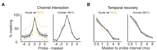
We agree that non-significant group-level slopes indicate that CI-evoked tonotopy is weaker than tone-evoked tonotopy, and we now emphasize this point. At the same time, the data exhibit systematic structure: for both ERP and HG, mean spatial correlations decline monotonically with increasing CI channel separation (Fig. 2B,G). We also directly compared spatial correlations at the extremes of stimulus separations (1 vs. ≥5-channel separation) and found a significant difference. This is updated in the manuscript as: “At the extremes, the spatial correlations were always higher for small vs. large tone separations (NH 0.5 vs ≥3.5 octaves, ERP: p<10-4, HG: p<10-4 Student’s one-tailed t-test) and electrode separations (CI 1 vs ≥5 electrodes, ERP: p=0.01, HG: p=0.04).”. Together with the strong deviation from shuffled maps in the vector-strength analysis (Fig. 2E), we argue that analysis of spatial correlations indicates that CI-evoked maps are not random but reflect a coarse underlying gradient. In addition, as tone-evoked maps exhibit tonotopy, we asked if CI stimulation itself is at least spatially tuned in the periphery. Using ECAPs with a forward-masking paradigm (new Supplemental Fig. 1), we show that probe-evoked ECAPs are significantly more suppressed by adjacent than by distant maskers (N = 3), demonstrating functional spatial tuning of CI electrodes in the cochlea. We have also replotted these results in comparison with the same measurements from a human CI user (Author response image 1). This supports the interpretation that peripheral input is spatially specific and that the weaker cortical cochleotopy likely reflects the properties and resolution of iEEG and acute CI stimulation rather than a complete absence of spatial organization. Overall, the new comparative figures and analyses are intended to make transparent that (i) iEEG robustly captures tonotopy for acoustic tones, and (ii) CI-evoked CI-evoked responses exhibit coarser, but statistically non-random, cochleotopic organization.
Author response image 1.
Here, we compare data from the new Supplemental Figure 1C,D with human data (N=1) for spatial & temporal tuning in the periphery, as assessed by forward masking ECAP measurements. A) Spatial tuning functions were averaged across all probe electrodes and 3 animals (left) and 1 human subject (right) (black, mean; gray: s.e.m..; orange, average of individual subjects). B) Temporal tuning functions were averaged across all probe electrodes and 3 animals (left) and 1 human subject (right) (black, mean; gray, s.e.m.; orange, average of individual subjects). Note: human subject is the first-author, a long-term cochlear implant user (>10 years) with significant open set speech perception.
(2) The statistical approach is inappropriate where pairing is incomplete: a Student's paired two-tailed t-test is used despite not all data being paired; a linear mixed-effects model would be more suitable, whereas an unpaired test risks reduced power.
We agree with this suggestion. As the reviewer notes (also raised by Reviewer 3), our original analyses did not fully exploit the partially paired structure of the data. In the initial submission we used paired t-tests when animals contributed both normal-hearing (NH) and CI measurements, which meant that animals with only NH or only CI data were excluded from those tests.
To address this, we have re-analyzed all NH vs. CI comparisons using linear mixed-effects models that incorporate both paired and unpaired observations within a single framework. This approach allows us to (i) include all available animals, (ii) appropriately account for within-animal dependence when both conditions are present, and (iii) align the statistical tests with the data shown in the figures. In nearly all cases, the mixed-effects models confirm our original conclusions. Two comparisons that were previously non-significant are now significant in the positive direction: Fig. 2E (p = 0.048) and Fig. 6F (p = 0.027, linear mixed-effects models). We have updated the manuscript to report these values and to clarify the use of mixed-effects modeling in the methods under the section titled, “Linear mixed effects modeling.”
(3a) Given the surgical complexity, objective verification of implantation and deafening is needed (e.g., eABRs for implant function and post-deafening ABR thresholds)”
We agree that objective verification of both implant placement and deafening is critical, particularly given the surgical complexity of multichannel CI implantation in rats. Note that we previously extensively documented deafness in our cochlear implant rats with eABRs, histology of hair cell counts, and behavior (turning the implant off and seeing performance drop to chance). As we argued in Glennon et al. Nature 2023, the primary outcome measure and definition of deafness is behavioral, as anatomical and physiological markers are correlates of functional deafness but ultimately deafness must be defined in terms of behavioral performance. This is described in more detail below.
We agree that objective verification of both implant placement and deafening is critical, particularly given the surgical complexity of multichannel CI implantation in rats. Note that we previously extensively documented deafness in our cochlear implant rats with eABRs, histology of hair cell counts, and behavior (turning the implant off and seeing performance drop to chance). As we argued in Glennon et al. Nature 2023, the primary outcome measure and definition of deafness is behavioral, as anatomical and physiological markers are correlates of functional deafness but ultimately deafness must be defined in terms of behavioral performance. This is described in more detail below.
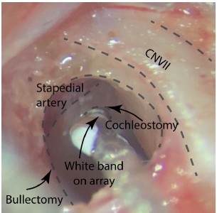
Implant placement: Our primary concern during surgery is to ensure that the CI array is correctly positioned along the cochlear spiral toward the apex. As shown in Author response image 2, once the bulla is opened and the cochleostomy is made at the junction of the temporal bone and the stapedial artery, the orientation of the cochlear spiral is clearly visible under the surgical microscope. We advance the 8-channel array only in the apical direction, and we require that all 8 electrodes pass through the cochleostomy. A complete insertion of all 8 electrodes cannot be achieved with a basal-ward trajectory, so full insertion provides a strong anatomical confirmation that the array is directed apically. The white band on the array, visible just basal to the cochleostomy (Author response image 2), serves as a consistent visual marker of complete insertion. We have added text and this figure to the Methods to clarify these criteria, “We required that all eight electrodes pass through the cochleostomy, confirming that the array was inserted in the direction of the apex.”
Verification of deafening: We also share the reviewer’s concern about confirming profound hearing loss, particularly because some CI animals were presented acoustic tones to drive individual channels. We used the same mechanical-only deafening procedure described and validated in our previous work (King et al., 2016; Glennon et al., 2023), which was chosen to minimize systemic side-effects and maximize post-surgical survival, validated in three ways:
- Histology: In N=4 deafened animals, inner hair cell loss was ~50% and outer hair cell loss was near complete at almost 100% in all animals.
- Physiology: For N=14 rats, acoustic ABRs were substantial before deafening but statistically similar to baseline noise after deafening.
- Behavior: For N=16 deafened rats, behavioral performance with implant on was d′: 1.7±0.1, but when implant was turned off in a subset of sessions, performance dropped to chance (d′: −0.05±0.1, P < 0.0001).
Author response image 2.
Visual confirmation of a successful electrode insertion. The direction of an 8-channel array being implanted toward the apex is clear under microscope. Full insertion of all 8 channels is further confirmed by the white band’s (located after basal electrode) proximity to the cochleostomy.
This combination of histological, physiological, and behavioral evidence indicates that the mechanical-only deafening protocol produces profound hearing loss, with no functionally relevant residual hearing at intensities equal to or greater than those used in our study (70 dB SPL). Given this prior validation under identical surgical and experimental conditions, we are confident that our CI animals were effectively deafened and that the iEEG responses we report are driven by the implant rather than by residual acoustic hearing. We now clarify this in the Methods and explicitly cite our validation: “(mechanical only, as described and validated in Glennon et al. 2023).
(3b) One CI animal did not learn the task (Fig. 1C), potentially reflecting implantation efficacy.
Good point, thanks. For both humans and rats, cochlear implant performance can be highly variable, reflecting a number of factors in terms of device performance, training efficacy and motivation, or other technical or biological sources of heterogeneity. We note however that not all animals included in this study were behaviorally trained, and wanted to show the full range of variable performance for the subset of animals that were trained (N=4 typical hearing and N=3 cochlear implant rats, one of the 4 trained animals lost the implant before it could be re-trained on the cochlear implant version of the task). We now highlight this range of performance variability in the results section and explain why N=4 normal-hearing and N=3 cochlear implant rats.
(4) The behavioural paradigm and cohort accounting are unclear: Figure 1C shows four NH-trained rats, yet subsequent analyses include only two NH-trained animals, which is confusing.
We have now clarified the relation between the behavioral cohort and the iEEG cohort in the revised manuscript. The key point is that the animals in Figure 1C are defined by their behavioral training history (NH vs CI training), whereas inclusion in the iEEG analyses is defined by the specific stimuli collected during acute recordings, and these two categorizations are not always the same. In total, four rats underwent both iEEG recordings and behavioral training. Of these four, three were subsequently deafened, implanted with chronic CIs, and trained on the CI-driven task (Fig. 1C). With respect to the acute iEEG experiments, we obtained tone-only iEEG in 1 animal, CI-only iEEG in 2 animals, and both tone- and CI-evoked iEEG in 1 animal.
Thus, the “NH-trained” label in Figure 1C refers to behavioral training status, not to the stimulus conditions used during iEEG recordings. All iEEG measurements were acute and performed immediately after surgery (for CI animals) or in the normal-hearing condition, before any CI behavioral training. Consequently, the behavioral cohort in Figure 1C is larger than the subset of animals that contributed to specific iEEG contrasts in later figures, which explains why some panels include only two NH animals.
To clarify this, we have added a new Supplementary Figure 2 that provides a timeline for each animal, indicating when behavioral training occurred, when deafening and implantation occurred, and which stimulus conditions (tones vs CI) were used for each iEEG recording. We kept this figure in the Supplementary section because the focus of the manuscript is on evoked iEEG measurements rather than behavior, but the revised text now explicitly refers to this schematic when describing the cohorts “The combinations of animals that underwent behavioral training and acute iEEG measurements are shown in Supplemental Fig. 2.”
(5) Methods lack essential details: specify acoustic stimulus types and intensities, CI stimulation parameters (e.g., current/charge per phase, phase width, rate, loudness setting), and the recording state (awake vs. anaesthetised), which is only implied in the discussion.
We agree that these details are essential, and Reviewer 3 raised similar concerns about methodological clarity. We have now expanded the Methods to specify the acoustic stimuli, CI stimulation parameters, and recording state.
Acoustic stimuli: We now describe the acoustic stimulus set in the Methods, which references Insanally et al. (2016). Briefly, tones were pure sinusoids spanning frequencies from 1.4 to 32 kHz (half octave spaced), presented at 70 dB SPL with a duration of 50 ms with 2ms cosine-squared ramps and at a pseudorandom sequence of 1.25 Hz. These parameters are now updated in the methods under “Stimulus presentation for cortical sensory mapping in normal hearing rats.”
CI stimulation parameters: CI stimulation used standard clinical-style monopolar mappings. We now specify in the Methods that pulses were biphasic, charge-balanced, with 8 µs interphase gaps and 25 µs /phase (total pulse width = 58 µs); stimulation rate was 900 pulses per second (pps); and current amplitude (and thus charge per phase) was set individually for each electrode based on its ECAP threshold. All stimulation levels were within normal and safe limits: charge densities remained below the Shannon limit and within the electrochemical “water window.”
Loudness setting: In this study, CI stimuli were presented primarily at a single level—each electrode was stimulated at its ECAP threshold level for the tone-to-CI mapping experiments. We have added these details in the methods under the “Stimulus presentation for cortical sensory mapping in cochlear implanted rats” subsection.
Recording state: All iEEG recordings reported in the manuscript were acute and performed under anesthesia. This is now stated explicitly at the start of the Methods section.
(6) Plasticity and training effects warrant further consideration: although the manuscript reports no difference between naïve and trained rats, Figure 3 suggests greater across-trial variability for CI than NH that is not evident in the trained subset; examining relationships among behavioural performance, decoder performance, across-trial variability, and training duration would strengthen interpretation.
We agree that plasticity and training effects are central questions for cochlear implant research and that iEEG is well suited to study how cortical representations evolve with CI use. However, the current dataset was collected mainly to compare cortical encoding of acoustic versus CI stimulation under matched, acute conditions (not necessarily after behavioral training with the implant, and we note that most studies of physiological responses to cochlear implant function in non-human species also do not incorporate aspects of training). All CI-evoked iEEG recordings were obtained immediately after implantation, before any CI-based behavioral training. As a result, any training effects reflected in the iEEG data can only arise from prior normal-hearing training, not from experience with CI stimuli themselves. Only a small subset of animals (N = 3 of 10) underwent behavioral training with cochlear implants, and their training histories (duration, performance levels, CI hardware status) are not uniform. This yields insufficient statistical power to meaningfully examine correlations among behavioral performance, decoder performance, across-trial variability, and training duration. While we note the reviewer’s observation that across-trial variability appears qualitatively different in the small, trained subset, we do not believe the current data justify strong conclusions about training-related plasticity.
(7) Differentiating the CI rats stimulated directly or through the microphone of the speech processor -at least in the figures - would be useful to allow the reader to assess whether both stimulation strategies give rise to similar results.
We agree that it is important to distinguish between rats stimulated directly via CI hardware and those stimulated acoustically through a speech processor. We now show in new Supplementary Figure 2, which animals received direct electrical stimulation and which were driven acoustically through the processor microphone. We also now plot tonotopic and cochleotopic maps for all CI animals in Supplementary Figure 3, with the stimulation mode indicated for each animal. As discussed in our response to comment #2 of Reviewer 3, we also provide validation that acoustic tones can be used to selectively drive individual electrodes via the speech processor. However, the sample sizes for the two stimulation strategies are small (N = 4 rats with direct CI stimulation, N = 3 rats with acoustic CI stimulation). For this reason, we have chosen not to draw strong statistical conclusions about differences between direct vs acoustic CI stimulation in the present manuscript.
(8) Typographical error at the end of the introduction ("To this end we have designed and manufactured..."), and in the first paragraph of the Discussion ("...that both that...").”
Thanks, we have updated the manuscript accordingly.
(9) Inconsistent terminology: use a single form (e.g., "normal-hearing") throughout.
Good suggestion, thanks. We have updated all main manuscript to only use normal-hearing. We found and changed two instances in which we used the acronym NH in lieu of normal-hearing, once early in the results section and once in the legend for Figure 3.
(10) In Figure 3D (temporal), there appears to be an extra data point for the NH-trained group.
Thank you for flagging this mis-labeling, which Reviewer 3 also pointed out. We have switched the appropriate data point in Figure 3D from ‘trained’ to ‘naïve’.
(11) In Figure 4D, the yellow line is not defined; based on Figure 6D, it likely represents shuffled/chance performance and should be labeled accordingly (including beneath the chance line on the plots).
We have updated Figure 6 to indicate that the yellow line does indeed reflect shuffled/chance.
(12) Figure 8 would benefit from a control demonstrating that poor cross-modal decoding reflects train-test distribution differences rather than weak decoders (e.g., train on a subsample of NH and test on held-out NH), and from reporting decoding on raw ERP/HG features in addition to TCA-derived data.
Good suggestion, thanks; we have now added this control. We agree that a positive control is necessary to show that poor tone→CI decoding reflects differences of underlying representations rather than a failure of the decoder or modeling approach. (Reviewer 2 raised the same point.)
To validate our cross‑modal analysis pipeline, we re‑implemented the full procedure used in Figure 8, but instead of training on tone‑evoked responses and testing on CI‑evoked responses, we trained and tested on independent sets of tone‑evoked trials from the same animals (tone→tone). For each tone in each animal, we withheld 10 trials as a test set. Using the remaining trials, we fit the original TCA model to obtain spatial and temporal factors (Fig. 8A). We then fixed these factors and re‑optimized only the trial factors on the withheld tone‑evoked trials (Fig. 8B). The LDA decoder was trained on the trial factors from the original TCA fit and tested on the re‑optimized trial factors from the withheld trials, using the same classification pipeline as in the main analysis.
As shown in the top panels of Figure 8C,D, this positive control yielded robust tone→tone generalization: predicted tone frequencies closely matched the actual tones, decoder performance was significantly above chance, and prediction errors were tightly clustered around the true stimulus, indicating that the decoder was tuned to tone frequency. In contrast, when we trained on tone‑evoked responses and tested on CI‑evoked responses, information transfer was markedly reduced (Fig. 8E-G).
These results demonstrate that the TCA+decoder pipeline can reliably transfer information across independent tone‑evoked datasets, confirming that the method captures shared structure when it exists. The poor cross‑modal transfer between tone‑ and CI‑evoked activity therefore is unlikely to be due to a weak decoder or to a failure of the modeling pipeline, but instead reflects a genuine mismatch between CI and sound representations in auditory cortex. We have updated Figure 8 and the Results section to describe this positive control analysis and clarify the interpretation.
(13) Perception and interpretation of signals are mentioned several times in the introduction, although perception is not explored in the manuscript (only neuronal processing). This might be confusing.
We appreciate the need to distinguish between neuronal encoding and perception. We also feel we have been careful not to invoke relationships to perception when presenting analyses on iEEG measurements, but we did identify an opportunity to further clarify this distinction between neuronal processing and perception by adding text in the intro, as follows “for the auditory system to interpret patterns of evoked neural activity and inform downstream auditory areas.”
(14) Figure 1C. Why is the performance of CI rats so much lower than what was previously published (Glennon et al., 2023)? Did the training duration change?
The three animals that were behaviorally trained on the normal-hearing (pre-deafening) and cochlear implant task (post-deafening) are within the distribution of the full set of animals from Glennon et al. (2023). However, we note that for Glennon et al. (2023), as one of our behavioral criterion was days to d’ > 1, animals were trained daily until reaching that level and not included in the initial data set if they did not reach that level. However, as we were including animals in this study of iEEG responses that were not trained at all, we felt it appropriate to include this third animal as well, that was trained just for 3 days before recordings were made. The two other animals were trained for 9 and 13 days. We have now included this information in the methods.
(15) The p-values = 0.5 should be given with an additional digit.
We previously rounded to the nearest single decimal digit, for all p-values greater than 0.10. We have updated the figures and manuscript text to ensure precision at least to the second digit.
Reviewer #2 (Recommendations for the authors):
We thank the Reviewer for their thoughtful comments on our study.
(1) Less noisy recording methods based on spike detection would provide stronger claims.
We agree that spike recordings, particularly isolated single-unit activity, are powerful for testing hypotheses about sensory encoding in auditory cortex, and we plan to incorporate such approaches in future work. However, our decision to use iEEG arrays in the present study was deliberate and central to the scientific and translational goals of the project.
First, iEEG and related population-level approaches such as scalp EEG (e.g., Lalor and Foxe, 2010; O’Sullivan et al., 2015) and fNIRS (e.g., Bortfeld et al., 2009; Peelle, 2017) are widely used in humans and have been highly successful in decoding sound- and speech-evoked responses, revealing fundamental principles of how sound and speech are encoded in the human brain. Because speech is uniquely human and cochlear implants are primarily designed to restore speech perception, aligning our recordings with clinically relevant, human-used modalities enhances the translational relevance of our work.
Second, iEEG arrays provide distinct advantages over modern multi- and single-unit electrophysiology. Even with high-density probes, the spatial sampling of neuronal activity does not match the coverage of the 60-channel iEEG arrays used here, which span large extents of auditory cortex. One might instead consider optical methods such as calcium imaging to interrogate topographical encoding at single-neuron and mesoscale resolutions, as has been done in normal-hearing mice (Romero and Hight et al., 2019). However, calcium signals are intrinsically slow, limiting access to the temporal precision that is critical for CI encoding, and these tools are unlikely to be available in humans in the foreseeable future, substantially reducing their translational value.
Using iEEG arrays, we show that CI-evoked responses are topographically organized, consistent with prior work (Klinke et al. 1999, Bierer and Middlebrooks 2002, Middlebrooks and Bierer 2002, including Adenis et al., 2024 now referenced in the manuscript). Our study extends these findings by exploiting simultaneous recordings across both spatial and temporal domains, which are essential for several key analyses (Figs. 3-8), including quantification of trial-by-trial variability, decoding of stimulus identity from single trials, and cross-modal comparisons between normal-hearing and CI-evoked iEEG responses.
Thus, we believe that the strength of this study is due to, rather than in spite of, its use of iEEG arrays. This approach uniquely allows us to test hypotheses about CI encoding across cortical topography and time using a modality that is directly translatable to human research and clinical practice. In response to the reviewer’s concern, we have also (i) improved the statistical treatment of our data (by adopting linear mixed-effects models that incorporate both paired and unpaired observations), (ii) added additional positive controls (see response to comment #2), and (iii) collected new data that further validate our rodent CI model. Together, these additions strengthen the support for our conclusions while preserving the key advantages of the iEEG-based approach.
(2) A positive control is necessary to claim the mismatch between CI and sound representations.
We agree. We now have added a positive control specifically designed to validate our cross-modal analysis pipeline in our revised manuscript. As also suggested by Reviewer 1, the goal was to test whether our method can successfully transfer information when the training and test datasets are matched in modality (tone→tone), thereby ensuring that the observed failure of cross-modal transfer (tone→CI) is not an artifact of the analysis.
To do this, we re-implemented the full pipeline used in Figure 8, but instead of training on tone-evoked responses and testing on CI-evoked responses, we trained and tested on independent sets of tone-evoked trials from the same animals. For each tone in each animal, we withheld 10 trials as a test set. Using the remaining trials, we fit the original TCA model to obtain spatial and temporal factors (Fig. 8A). We then fixed these factors and re-optimized only the trial factors on the withheld tone-evoked trials (Fig. 8B). The LDA decoder was trained on the trial factors from the original TCA fit and tested on the re-optimized trial factors from the withheld trials, using the same classification pipeline as elsewhere in the manuscript.
As shown in the top panels of Figure 8C,D, this positive control yielded robust tone→tone generalization: predicted tone frequencies closely matched the actual tones, decoder performance was significantly above chance, and prediction errors were tightly clustered around the true stimulus, indicating that the decoder was tuned to tone frequency. In contrast, when we trained on tone-evoked responses and tested on CI-evoked responses, information transfer was markedly reduced and not different from shuffled controls (Fig. 8E-G).
These results demonstrate that the TCA+decoder pipeline can reliably transfer information across independent tone-evoked datasets, confirming that the method captures shared structure when it exists. The poor cross-modal transfer between tone- and CI-evoked activity therefore cannot be attributed to a failure of the modeling pipeline but instead reflects a mismatch between CI and sound representations in auditory cortex. We have updated Figure 8, the methods, and the results section to include this new important analysis.
Reviewer #3 (Recommendations for the authors):
We thank reviewer 3’s appreciation for study design and the appropriateness of analyses taken. We also appreciate the recognition of noteworthiness, specifically that stimulus identity can be decoded on a single-trial basis and of the potential benefit of using central decoders in clinical settings.
(1a) Animal heterogeneity: It is difficult to keep track of the animals used in this study, and some received a different protocol of stimulation (sounds through the speech processor vs. direct stimulation) and were also trained in a behavioral task using different target stimuli (4kHz vs. 22.6kHz, also no mention of the CI electrode used as a target).
We have now clarified the animal cohorts and stimulation protocols in our revised manuscript. We added a new Supplementary Figure 2 that schematizes, for each animal if it underwent behavioral training with pure tones in the normal-hearing condition, if tone-evoked iEEG measurements were collected, if CI-evoked iEEG measurements were collected (and whether stimulation was direct or via the speech processor), and if it subsequently received CI-based behavioral training. Regarding the behavioral targets, we now specify in the Methods that for normal-hearing training, the target stimulus was a 22.6-kHz pure tone. For CI-trained animals, the target was either CI channel 3 (n = 2 rats) or CI channel 4 (n = 1 rat). Details about stimuli targets during behavior have been added to the methods section under “Behavioral training for tone and implant channel detection.”
(1b) There is no comparison of the CI maps from rats tested with the speech processor and directly stimulated. How different were they? Was the frequency allocation of each electrode the same for each animal? Since data might already have intrinsic variability because of the grid placement, the mechanical deafening, and the cochlear implantation in each animal, such heterogeneity in the 'background' and stimulation protocol might blur the authors' results.
Our study focuses on cortical encoding of single-channel CI stimulation, so it is indeed important to ensure that the stimuli are effectively delivered by a single electrode, regardless of whether they are driven acoustically via the speech processor or by direct electrical stimulation.
Stimulation mode and frequency allocation: The project began with single-channel stimulation achieved by presenting pure tones to the speech processor (N=3 animals) and later transitioned to direct programmatic control of individual electrodes (N=4 animals) to simplify the experimental setup. In both cases, the goal was to activate only one CI channel at a time.
For the programming speech-processor animals, the validation protocol described in Glennon et al. (2023) is as follows:
- Set the number of active channels in the processor to 1 (the clinical default is 8) to avoid spectral spread across electrodes.
- Disabled all additional signal-processing strategies (e.g., Scan, ASC, ADRO, SNR-NR, WNR).
- Used customized frequency allocation tables that mapped narrow frequency bands to individual electrodes, as shown in Glennon et al., 2023, Extended Data Fig. 2.
To confirm that a given tone drove only the intended electrode, we recorded tone-evoked electrodograms—measurements of the output at each electrode—and verified that only the targeted channel was active (Glennon et al., 2023, Extended Data Fig. 2). Thus, although the initial CI drive was acoustic, the effective stimulation at the array was restricted to a single electrode with a well-defined frequency allocation.
For the direct-stimulation animals, we used the same underlying frequency allocations to choose which electrode to stimulate, but the pulses were delivered programmatically rather than via the speech processor. In both modes, the center frequency associated with each electrode was therefore defined consistently across animals, and stimulation was confined to one channel at a time.
Comparison of maps across stimulation modes: We now explicitly indicate the stimulation mode (speech-processor vs direct) for each CI animal in Supplementary Figure 2 and plot the maps for all animals in Supplementary Figure 3. Qualitatively, the spatial organization of CI-evoked maps is similar across the two stimulation strategies; we do not observe systematic differences in map structure that would suggest large biases introduced by the stimulation mode. However, the sample sizes for each group are small (N = 3 speech-processor, N = 4 direct). For this reason, we have not performed formal between-mode statistics and instead treat stimulation mode as a source of minor heterogeneity, alongside inevitable variability from grid placement, mechanical deafening, and cochlear insertion. Given the electrodogram validation (Glennon et al., 2023, Extended Data Fig. 2) and consistent frequency allocation tables, we are confident that both approaches produce single-channel activation with comparable effective frequency assignments.
(1c) The number of animals used is also confusing. The authors report 7 NH and 7 CI animals (14 total), 4 NH and 3 CI were trained before being implanted (so 3 naïve NH and 4 naïve CI remain). Figure 1C reports that only 3 trained NH performed with the CI (let us call them 3 NH->CI). But then Figure 1E reports only 1 trained NH->CI and only 1 trained NH and 3 naïve NH that got implanted later. On the other hand, Figure 1E reports only 1 true naïve CI animal, the 3 others being naïve NH that got implanted. For the sake of clarity, I would encourage the authors to provide a timeline of the procedures/stimulation protocols coupled with a schematic distribution of the animals.
To address this, we have added a new Supplementary Figure 2 that provides, for each individual animal a chronological timeline (NH recordings, deafening, implantation, CI recordings); if it was behaviorally trained in the NH condition, the CI condition, or both; if CI stimulation was delivered via the speech processor or by direct electrical stimulation; and which stimulus conditions (tone-evoked iEEG, CI-evoked iEEG) were collected. This schematic makes it clear how the reported totals arise (7 NH and 7 CI for iEEG; 4 NH-trained and 3 CI-trained behaviorally) and shows which specific animals contribute to each panel in Figure 1 and to the later iEEG analyses. We now reference Supplementary Figure 2 in the Results when introducing the cohorts to guide readers through animal accounting.
(2a) Methods and statistics: Deafening is only mechanical, with no direct or postmortem proof that deafening was complete. The authors cite previous studies, but that would have been a good control to have since mechanical deafening isn't as accepted as the chemical deafening, like Neomycin, especially when some of your animals were stimulated with pure tones through the speech processor.”
We agree that rigorous verification of deafening is essential, particularly when some CI animals are driven acoustically through the speech processor. Ototoxic approaches (e.g., systemic or local neomycin) are one established method, but their effectiveness can be sensitive to dose and delivery, and they introduce systemic side-effects that can complicate long-term survival and recovery.
Our laboratory has used the mechanical deafening procedure since it was first described in King et al. (2016) and more recently in Glennon et al. (2023). In King et al., mechanical and ototoxic methods were combined, and we found that ototoxic methods provided no more additional robustness in deafening compared to mechanical lesion. Instead, the additional time required for ototoxic drug application reduced survival times in what was already a very complex and long surgical procedure for bilateral deafening and unilateral cochlear implantation.
In Glennon et al. (2023) we intentionally employed mechanical-only deafening to minimize side-effects while still achieving profound hearing loss in implanted animals. Glennon et al. (2023) provides an extensive validation of this mechanical-only protocol under the same surgical and experimental conditions as the present study. As we mentioned in our response to comment #3a of Referee 1, we assessed deafness through three measures:
Histology: In N=4 deafened animals, inner hair cell loss was ~50% and outer hair cell loss was near complete at almost 100% in all animals.
Physiology: For N=14 rats, acoustic ABRs were substantial before deafening but statistically similar to baseline noise after deafening.
Behavior: For N=16 deafened rats, behavioral performance with implant on was d′: 1.7±0.1, but when implant was turned off in a subset of sessions, performance dropped to chance (d′: −0.05±0.1, P < 0.0001).
This convergent anatomical, physiological, and behavioral evidence demonstrates that the mechanical procedure produces profound deafness, with no functionally relevant residual hearing at levels ≥90 dB SPL. Also as we mentioned in response to comment #3a of Referee 1, we believe that the behavioral criterion is most essential and also least common in the literature. Because the tones used to drive the speech processor in the current study were presented at 70 dB SPL, we have no reason to believe that residual acoustic hearing contributed to any of the CI-evoked responses we report.
We now cite these validation data explicitly in the methods under the section “Bilateral sensorineural hearing loss” as follows “(mechanical only, as described and validated in Glennon et al. 2023)” to make clear why we consider the mechanical-only approach sufficient for ensuring deafness in the present experiments.
(2b) What motivated the selection of 15 Principal Components for the PCA? That might need to be justified, maybe by scree plot or variance plot (Eigen Values or CEV), as if too many PCs are selected, you are at risk of losing information. Side comment for TCA: why is it important that the number of latent factors exceeds the number of tones or stimuli? Is there a way to justify this statement?
We thank the reviewer for raising this point. Our choice of 15 components/latent factors was motivated by both theoretical and empirical considerations, which are now made explicit in the manuscript.
For the PCA analyses, we selected 15 principal components for two reasons. First, because our decoder must discriminate between 10 tone conditions, we reasoned that providing at least as many dimensions as stimuli would be beneficial, while also allowing for the possibility that some components may carry little or no stimulus-selective information. We therefore chose a modest number of components that exceeded the number of tones (10) but avoided unnecessarily high dimensionality. Second, we empirically examined the variance explained as a function of the number of components. As shown in the new scree plots (Supplemental Fig. 4A), the cumulative variance explained enters a near-linear, low-slope regime beyond ~15 PCs, indicating diminishing returns for including additional components. Thus, 15 PCs capture a substantial fraction of the stimulus-related variance while minimizing the risk of overfitting and retaining a consistent dimensionality across animals.
For the TCA analyses, we used 15 latent factors to match the dimensionality used in PCA and to ensure that the latent space was sufficiently flexible to represent the 10 tone conditions without being under-parameterized. In practice, increasing the number of TCA components reduces reconstruction error (Williams et al., 2018), but with diminishing improvement beyond a certain point. We therefore systematically evaluated model error as a function of the number of latent factors and found that error decreased rapidly up to ~15 components and then plateaued (Supplemental Fig. 4B). This pattern parallels the PCA scree plots and supports 15 as a reasonable trade-off between model flexibility and parsimony.
We have updated the Results clarify these choices, as follows “The number of components (15) was chosen based on PCA scree plots (Supplemental Fig. 4A), which showed that explained variance entered a near‑linear, low‑slope regime beyond this point demonstrating a similar plateau in reconstruction error (Supplemental Fig. 4B).”
(2c) Legend of Figure 2E, J states that a Student's paired t-test was used, meaning that only the 'linked' points of the graph were used (thus, comparing only animals that got tested NH then implanted). This is usually the same across the manuscript. Why not include all the points with an unpaired t-test? Otherwise, why are all the points plotted if they serve no purpose? This choice should be justified.
We agree with this concern, which was also raised by Reviewer 1. We have revised our statistical approach accordingly in our revised manuscript. In the original submission, we used paired t-tests when animals contributed both normal-hearing (NH) and CI data, which meant that animals with only NH or only CI measurements were excluded from those comparisons even though they were shown in the plots.
To address this, we have re-analyzed all normal-hearing vs. CI comparisons using linear mixed-effects models that include both paired and unpaired data within a single framework. This approach ensures that every plotted data point contributes to the statistical tests, properly accounts for within-animal dependence when both conditions are present, and avoids the loss of power that would arise from either paired-only or purely unpaired tests.
The mixed-effects results are consistent with our original interpretations, with two comparisons becoming significant in the updated analysis: Fig. 2E (p = 0.048) and Fig. 6F (p = 0.027). We have updated the Results and figure legends to describe the use of mixed-effects models and to report these revised p-values. Together with the new tonotopy and cochleotopy analyses described above, these changes strengthen the statistical support for our conclusions without altering the overall interpretation of the data.
(2d) Side comment: There are inconsistencies on the bar plots of Figure 6C (Missing a purple point) and Figure 3D (Temporal has 3 purple points).
Thank you for flagging this mis-labeling (which Reviewer 1 also noticed). We have correctly updated the appropriate data point from trained to naive for Fig. 3D and from naive to trained for Fig. 6C.
(3a) Pure tones and CI-evoked responses maps: It is the reviewer's understanding that Figure 2 is an averaged representation for all animals. Why is the tonotopic shift so dim for ERPs? The averaged maps aren't very convincing. How were the gradients on an animal-to-animal basis since Figure 2D is only an example animal? Also, everything has been evaluated at 70dB, where selectivity might not be best. It would have been easier to follow the tonotopic gradient at the CFs where contrasts are higher.
We agree that the strength and interpretation of tonotopy/cochleotopy in our iEEG data needed to be presented more clearly. Reviewer 1 raised closely related concerns, and we have substantially expanded the analyses and explanations in response. Here we highlight the points that address your specific questions.
Single-animal vs. averaged maps: We included both exemplar maps and population summaries in Figure 2. The panels analogous to Figure 2D show single-animal best-frequency (BF) or best-channel maps; these were chosen because they exhibit clear, interpretable gradients. In the exemplar shown, there is a local high-frequency (HF) region along the medial edge of the array that transitions to lower frequencies toward the rostral edge. For CI-evoked best-channel maps in the same animal, we observe a parallel pattern in which basal electrodes (e.g., electrode 8, representing higher frequencies) occupy the HF region and apical electrodes (e.g., electrode 1, lower frequencies) occupy the LF region.
Averaged ERP maps, by contrast, necessarily blur some of this structure because iEEG is a summed field potential and animal-to-animal differences in array placement, cochlear insertion depth, and anatomy introduce variability. We have softened the language in the text to reflect that ERP-based tonotopy is coarse and weaker at the population level, while emphasizing that robust gradients are evident in single animals and in HG-based measures.
Quantitative assessment across animals: To move beyond visual impressions, we added quantitative analyses that mirror those used in Romero and Hight et al. (2020) for calcium imaging data (Romero and Hight et al. 2020 and Fig. 2). For each map we computed local tonotopic gradient vectors at every pixel and summarized their magnitude/direction on a unit circle, then compared the mean vector strength to shuffled maps. Applied to our BF and best-channel maps, this analysis shows that both are significantly more ordered than shuffled controls (p < 10-10), indicating that the maps are tonotopic/cochleotopic rather than random, despite the apparent dimness of the gradients in some averaged ERP plots. These new results are described in the revised manuscript and shown in Romero and Hight et al. 2020 and Fig. 2.
Effect of intensity (70 dB SPL) and “dim” gradients: We agree that stimulus level influences the apparent sharpness of tonotopy. Higher intensities tend to broaden tuning and compress the dynamic range of BF maps. As we now discuss in more detail (adapted from our response to Reviewer 1), tones were presented at 70 dB SPL, so we expect maps to emphasize mid-frequency regions (around 8 kHz) and to show somewhat broader tuning than maps derived at threshold. For CI stimulation, we used ECAP thresholds to set intensity, which is effective in our preparation because animals can robustly discriminate individual electrodes and these electrodes evoke clear cortical activity (King et al., 2015; Glennon et al., 2023).
In summary, we clarified which panels in Figure 2 show single-animal exemplars vs population summaries, added quantitative analyses demonstrating spatial correlations are greater for adjacent stimuli compared to far-apart stimuli, and expanded the discussion of how recording modality and stimulus level influence the visibility of tonotopic gradients. These changes are intended to make the evidence for tonotopy/cochleotopy in our iEEG data (and its limitations) more transparent.
(3b) Since new experiments might not be available, it is the reviewer's suggestion to add a supplementary figure showing a couple of animal examples following the format of Figures 2A and 2C that have more contrasted gradients to strengthen the group data. In the case of the CI-evoked responses map, this might also provide another argument to dismiss the potential monopolar smearing.
Good suggestion, thanks. We now include a new Supplementary Figure 3 that shows additional single-animal examples for both tone-evoked and CI-evoked maps, following the same format as Figure 2C.
Regarding monopolar stimulation, we agree that monopolar configurations are expected to be less spatially specific than bipolar or multipolar modes because current returns to an extracochlear reference electrode, potentially broadening the spread of excitation. We nevertheless chose monopolar stimulation because it is the predominant clinical configuration in human CI users and therefore most relevant for translational purposes. We acquired ECAP measurements of peripheral (spatial and temporal) tuning via a forward masking paradigm and demonstrate that monopolar is effectively tuned (Supplemental Fig. 2). Together with additional single-animal maps in Supplementary Figure 3, together with our vector-strength analysis (Romero and Hight et al. 2020 and Fig. 2), demonstrate that even under acute monopolar stimulation we observe structured cochleotopic organization in cortex, rather than the fully smeared patterns one might expect if monopolar spread completely dominated.
We also note that all CI-evoked iEEG measurements were made acutely, immediately after implantation and before any CI-based behavioral experience. It is possible that with longer-term use and plasticity, cortical cochleotopy could become sharper than what we observe here under acute conditions. In this sense, our data provide a conservative baseline showing that even at the earliest stages of CI use, monopolar stimulation already engages tonotopically selective regions of auditory cortex. A longitudinal comparison of acute versus chronic maps would be an interesting direction for future work but is beyond the scope of the current study.
(3c) Side comments: The legends of Figures 2D and 2I should mention that this is an animal example and not group data, as the rest of the figures are group data.
Thank you for this suggestion to improve figure clarity. We have updated all of our figures, where appropriate, to indicate whether data are single or groups of animals.
(3d) In general, some of the legends should be revised because they are sometimes too "strong". As an example, Figure 3B, D legend states: "Variability of iEEG measurements across trials (root mean square, rms) was consistently higher for cochlear implant-evoked compared to tone-evoked activity", despite three of the statistical tests being non-significant. The manuscript is correct, on the other hand.
Good point. We revised the legend for Figure 3 to be consistent with the figure and the manuscript.
(3e) The example spatial map given in Figure 3A for CI might not be the best choice since it is showing a pretty reliable trial-by-trial response, while your group data proves the opposite.
We understand the reviewer’s concern and agree that the exemplar CI map in Figure 3A appears relatively reliable on a trial-by-trial basis. This example was chosen deliberately from an animal in which we had both NH- and CI-evoked iEEG recordings, so that the reader could visually compare the two conditions within the same preparation. In this animal, as in the group data, the differences between NH and CI trial-by-trial responses are subtle rather than dramatic.
Our group-level analysis shows that the RMS error across trials is consistently higher for CI-evoked than for NH-evoked responses, but the absolute differences are small (< 0.1) and relatively uniform across animals. The spatial maps plotted in Figure 3A are representative of this pattern: both conditions show reasonably robust evoked responses, with CI responses nonetheless showing slightly greater variability. To avoid implying a stronger qualitative difference than is supported by the data, we have revised the text to emphasize that (i) CI-evoked responses remain clearly detectable on single trials, and (ii) the key effect is a small but consistent increase in variability across animals, as captured by the RMS error metrics, “We noted that the differences were qualitatively subtle (Fig. 3A, right panel), they were consistent across animals (Fig. 3B).”
(4a) Decoders for CI stimulation Regarding CI stimulation, Pearson's correlations were truncated at a spacing of 5 electrodes. Likewise, none of the LDA classifiers show prediction for channels past CI-6. Again, that choice should be justified, or the missing channels should be presented.
We truncated the correlation between electrodes at 5 because beyond that, the estimated means are significantly noisy. These estimated means are noisy because the number of data are significantly reduced, also significantly increasing the standard error. For example, for the maximum stimulus spacing, the number of pairwise correlations is at maximum the number of animals tested (i.e., N=7). We believe it’s important to be transparent, so we have included the non-truncated version of the figure here in this public review (Author response image 3). We leave the figures in the manuscript untouched but have updated the Figure 2 legend justify this selection of data.
Author response image 3.
Expanded figures for spatial correlations and LDA performance. A) The same data from manuscript Figure 2 are re-plotted but with expanded x-axes to include up to 4.5 octaves and 7 channels. Due to the smaller numbers of data at these points, the estimates for the mean spatial correlations are noisier. In all cases, the mean correlations are significantly higher for the first data point compared to the last 3 (NH, ERP p<0.001; NH, HG p<0.001; CI, ERP p=0.005; and CI, HG p=0.39, linear mixed effects models). B) The same data from manuscript figure 4 are re-plotted but with expanded x-axes to include up to ±3.5 octaves and ±6 channels.
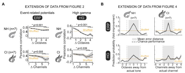
(4b) Finally, retrained PCA-LDA on spatial-only and temporal-only for CI are absent in Figure 3D. Since the authors were pretty consistent in showing both NH and CI alongside in the rest of the paper, it would be coherent to add the CI counterpart to Figure 3D, or maybe with a supplementary figure.
We agree that consistency can be improved by including classifiers for CI-evoked measurements, though presumably for Fig. 6C and not Fig. 3D. Figure 6 has been updated accordingly.
-
eLife Assessment
This valuable study compares auditory cortex responses to sounds and cochlear implant stimulation measured with surface electrode grids in rats. Beyond the reduced frequency resolution of cochlear implants observed previously, this study suggests key discrepancies between neuronal representations of cochlear stimulations and natural sounds. However, the evidence for this potentially interesting result is incomplete because there is a lack of evidence for the effectiveness of the comparison method. This study is of interest to researchers in the auditory neuroscience field and clinicians implementing treatments with cochlear implants.
-
Reviewer #1 (Public review):
Summary:
This manuscript addresses an important question: whether cortical population codes for cochlear-implant (CI) stimulation resemble those for natural acoustic input or constitute a qualitatively different representation. The authors record intracranial EEG (µECoG) responses to pure tones in normal-hearing rats and to single-channel CI pulses in bilaterally deafened, acutely implanted rats, analysing the data with ERP/high-gamma measures, tensor component analysis (TCA), and information-theoretic decoding. Across several readouts, the acoustic condition supports better single-trial stimulus classification than the CI condition. However, stronger decoding does not, on its own, establish that the acoustic responses instantiate a "richer" cortical code, and the evidence for orderly spatial organisation is …
Reviewer #1 (Public review):
Summary:
This manuscript addresses an important question: whether cortical population codes for cochlear-implant (CI) stimulation resemble those for natural acoustic input or constitute a qualitatively different representation. The authors record intracranial EEG (µECoG) responses to pure tones in normal-hearing rats and to single-channel CI pulses in bilaterally deafened, acutely implanted rats, analysing the data with ERP/high-gamma measures, tensor component analysis (TCA), and information-theoretic decoding. Across several readouts, the acoustic condition supports better single-trial stimulus classification than the CI condition. However, stronger decoding does not, on its own, establish that the acoustic responses instantiate a "richer" cortical code, and the evidence for orderly spatial organisation is not compelling for CI, and is also less evident than expected for normal-hearing, given prior knowledge. The overall narrative is interesting, but at present, the conclusions outpace the data because of statistical, methodological, and presentation issues.
Strengths:
The study poses a timely, clinically relevant question with clear implications for CI strategy. The analytical toolkit is appropriate: µECoG captures mesoscale patterns; TCA offers a transparent separation of spatial and temporal structure; and mutual-information decoding provides an interpretable measure of single-trial discriminability. Within-subject recordings in a subset of animals, in principle, help isolate modality effects from inter-animal variability. Where analyses are most direct, the acoustic condition yields higher single-trial decoding accuracy, which is a meaningful and clearly presented result.
Weaknesses:
Several limitations constrain how far the conclusions can be taken. Parts of the statistical treatment do not match the data structure: some comparisons mix paired and unpaired animals but are analysed as fully paired, raising concerns about misestimated uncertainty. Methodological reporting is incomplete in places; essential parameters for both acoustic and electrical stimulation, as well as objective verification of implantation and deafening, are not described with sufficient detail to support confident interpretation or replication. Figure-level clarity also undermines the message. In Figure 2, non-significant slopes for CI, repeated identification of a single "best channel," mismatched axes, and unclear distinctions between example and averaged panels make the assertion of spatial organisation unconvincing; importantly, the normal-hearing panels also do not display tonotopy as clearly as expected, which weakens the key contrast the paper seeks to establish. Finally, the decoding claims would be strengthened by simple internal controls, such as within-modality train/test splits and decoding on raw ERP/high-gamma features to demonstrate that poor cross-modal transfer reflects genuine differences in the underlying responses rather than limitations of the modelling pipeline.
-
Reviewer #2 (Public review):
Summary:
This article reports measurements of iEEG signals on the rat auditory cortex during cochlear implant or sound stimulation in separate groups of rats. The observations indicate some spatial organization of cochlear implant stimuli, but that is very different from cochlear implants.
Strengths:
The study includes interesting analyses of the sound and cochlear implant representation structure based on decoders.
Weaknesses:
The observation that responses to cochlear implant stimulation (stimulation) are spatially organized is not new (e.g., Adenis et al. 2024).
The claim that spatial and temporal dimensions contribute information about the sound is also not new; there is a large literature on this topic. Moreover, the results shown here are extremely weak. They show similar levels of information in the …
Reviewer #2 (Public review):
Summary:
This article reports measurements of iEEG signals on the rat auditory cortex during cochlear implant or sound stimulation in separate groups of rats. The observations indicate some spatial organization of cochlear implant stimuli, but that is very different from cochlear implants.
Strengths:
The study includes interesting analyses of the sound and cochlear implant representation structure based on decoders.
Weaknesses:
The observation that responses to cochlear implant stimulation (stimulation) are spatially organized is not new (e.g., Adenis et al. 2024).
The claim that spatial and temporal dimensions contribute information about the sound is also not new; there is a large literature on this topic. Moreover, the results shown here are extremely weak. They show similar levels of information in the spatial and temporal dimensions, and no synergy between the two dimensions. This is however, likely the consequence of high measurement noise leading to poor accuracy in the information estimates, as the authors state.
The main claim of the study - the mismatch between cochlear implant and sound representation - is not supported. The responses to each modality are measured in different animals. The authors do not show that they actually can compare representations across animals (e.g., for the same sounds). Without this positive control, there is no reason to think that it is possible to decode from one animal with a decoder trained on another, and the negative result shown by the authors is therefore not surprising.
-
Reviewer #3 (Public review):
Summary:
Through micro-electroencephalography, Hight and colleagues studied how the auditory cortex in its ensemble responds to cochlear implant stimulation compared to the classic pure tones. Taking advantage of a double-implanted rat model (Micro-ECoG and Cochlear Implant), they tracked and analyzed changes happening in the temporal and spatial aspects of the cortical evoked responses in both normal hearing and cochlear-implanted animals. After establishing that single-trial responses were sufficient to encode the stimuli's properties, the authors then explored several decoder architectures to study the cortex's ability to encode each stimulus modality in a similar or different manner. They conclude that a) intracranial EEG evoked responses can be accurately recorded and did not differed between normal …
Reviewer #3 (Public review):
Summary:
Through micro-electroencephalography, Hight and colleagues studied how the auditory cortex in its ensemble responds to cochlear implant stimulation compared to the classic pure tones. Taking advantage of a double-implanted rat model (Micro-ECoG and Cochlear Implant), they tracked and analyzed changes happening in the temporal and spatial aspects of the cortical evoked responses in both normal hearing and cochlear-implanted animals. After establishing that single-trial responses were sufficient to encode the stimuli's properties, the authors then explored several decoder architectures to study the cortex's ability to encode each stimulus modality in a similar or different manner. They conclude that a) intracranial EEG evoked responses can be accurately recorded and did not differed between normal hearing and cochlear-implanted rats; b) Although coarsely spatially organized, CI-evoked responses had higher trial-by-trial variability than pure tones; c) Stimulus identity is independently represented by temporal and spatial aspect of cortical representations and can be accurately decoded by various means from single trials; d) and that Pure tones trained decoder can't decode CI-stimulus identity accurately.
Strength:
The model combining micro-eCoG and cochlear implantation and the methodology to extract both the Event Related Potentials (ERPs) and High-Gammas (HGs) is very well designed and appropriately analyzed. Likewise, the PCA-LDA and TCA-LDA are powerful tools that take full advantage of the information provided by the cortical ensembles.
The overall structure of the paper, with a paced and exhaustive progress through each step and evolution of the decoder, is very appreciable and easy to follow. The exploration of single-trial encoding and stimulus identity through temporal and spatial domains is providing new avenues to characterize the cortical responses to CI stimulations and their central representation. The fact that single trials suffice to decode the stimulus identity regardless of their modality is of great interest and noteworthy. Although the authors confirm that iEEG remains difficult to transpose in the clinic, the insights provided by the study confirm the potential benefit of using central decoders to help in clinic settings.
Weaknesses:
The conclusion of the paper, especially the concept of distinct cortical encoding for each modality, is unfortunately partially supported by the results, as the authors did not adequately consider fundamental limitations of CI-related stimulation.
First, the reviewer assumed that the authors stimulated in a Monopolar mode, which, albeit being clinically relevant, notoriously generates a high current spread in rodent models. Second, comparing the averaged BF maps for iEEG (Figure 2A, C), BFs ranged from 4 to 16kHz with a predominance of 4kHz BFs. The lack of BFs at higher frequencies hints at a potential location mismatch between the frequency range sampled at the level of the cortex (low to medium frequencies) and the frequency range covered by the CI inserted mostly in the first turn-and-a-half of the cochlea (high to medium frequencies). Looking at Figure 2F (and to some extent 2A), most of the CI electrodes elicited responses around the 4kHz regions, and averaged maps show a predominance of CI-3-4 across the cortex (Figure 2C, H) from areas with 4kHz BF to areas with 16kHz BF. It is doubtful that CI-3-4 are located near the 4kHz region based on Müller's work (1991) on the frequency representation in the rat cochlea.
Taken together with the Pearsons correlations being flat, the decoder examples showing a strong ability to identify CI-4 and 3 and the Fig-8D, E presenting a strong prediction of 4kHz and 8kHz for all the CI electrodes when using a pure tone trained decoder, it is possible that current spread ended stimulating indistinctly higher turns of the cochlea or even the modiolus in a non-specific manner, greatly reducing (or smearing) the place-coding/frequency resolution of each electrode, which in turn could explain the coarse topographic (or coarsely tonotopic according to the manuscript) organization of the cortical responses. Thus, the conclusion that there are distinct encodings for each modality is biased, as it might not account for monopolar smearing. To that end, and since it is the study's main message and title, it would have benefited from having a subgroup of animals using bipolar stimulations (or any focused strategy since they provide reduced current spread) to compare the spatial organization of iEEG responses and the performances of the different decoders to dismiss current spread and strengthen their conclusion.
Nevertheless, the reviewer wants to reiterate that the study proposed by Hight et al. is well constructed, relevant to the field, and that the overall proposal of improving patient performances and helping their adaptation in the first months of CI use by studying central responses should be pursued as it might help establish new guidelines or create new clinical tools.
-
-
