Exploiting fluctuations in gene expression to detect causal interactions between genes
Curation statements for this article:-
Curated by eLife

eLife Assessment
By taking advantage of noise in gene expression, this important study introduces a new approach for detecting directed causal interactions between two genes without perturbing either. The main theoretical result is supported by a proof. Preliminary simulations and experiments on small circuits are solid, but further investigations are needed to demonstrate the broad applicability and scalability of the method.
This article has been Reviewed by the following groups
Discuss this preprint
Start a discussion What are Sciety discussions?Listed in
- Evaluated articles (eLife)
Abstract
Characterizing and manipulating cellular behavior requires a mechanistic understanding of the causal interactions between cellular components. We present an approach to detect causal interactions between genes without the need to perturb the physiological state of cells. This approach exploits naturally occurring cell-to-cell variability which is experimentally accessible from static population snapshots of genetically identical cells without the need to follow cells over time. Our main contribution is a simple mathematical relation that constrains the propagation of gene expression noise through biochemical reaction networks. This relation allows us to rigorously interpret fluctuation data even when only a small part of a complex gene regulatory process can be observed. We show how this relation can, in theory, be exploited to detect causal interactions by synthetically engineering a passive reporter of gene expression, akin to the established ‘dual reporter assay’. While the focus of our contribution is theoretical, we also present an experimental proof-of-principle to demonstrate the real-world applicability of our approach in certain circumstances. Our experimental data suggest that the method can detect causal interactions in specific synthetic gene regulatory circuits in Escherichia coli, confirming our theoretical result in a narrow set of controlled experimental settings. Further work is needed to show that the approach is practical on a large scale, with naturally occurring gene regulatory networks, or in organisms other than E. coli .
Article activity feed
-

-
-
-

eLife Assessment
By taking advantage of noise in gene expression, this important study introduces a new approach for detecting directed causal interactions between two genes without perturbing either. The main theoretical result is supported by a proof. Preliminary simulations and experiments on small circuits are solid, but further investigations are needed to demonstrate the broad applicability and scalability of the method.
-
Reviewer #2 (Public Review):
Summary:
This paper describes a new approach to detecting directed causal interactions between two genes without directly perturbing either gene. To check whether gene X influences gene Z, a reporter gene (Y) is engineered into the cell in such a way that (1) Y is under the same transcriptional control as X, and (2) Y does not influence Z. Then, under the null hypothesis that X does not affect Z, the authors derive an equation that describes the relationship between the covariance of X and Z and the covariance of Y and Z. Violation of this relationship can then be used to detect causality.
The authors benchmark their approach experimentally in several synthetic circuits. In 4 positive control circuits, X is a TetR-YFP fusion protein that represses Z, which is an RFP reporter. The proposed approach detected …
Reviewer #2 (Public Review):
Summary:
This paper describes a new approach to detecting directed causal interactions between two genes without directly perturbing either gene. To check whether gene X influences gene Z, a reporter gene (Y) is engineered into the cell in such a way that (1) Y is under the same transcriptional control as X, and (2) Y does not influence Z. Then, under the null hypothesis that X does not affect Z, the authors derive an equation that describes the relationship between the covariance of X and Z and the covariance of Y and Z. Violation of this relationship can then be used to detect causality.
The authors benchmark their approach experimentally in several synthetic circuits. In 4 positive control circuits, X is a TetR-YFP fusion protein that represses Z, which is an RFP reporter. The proposed approach detected the repression interaction in 2 of the 4 positive control circuits. The authors constructed 16 negative control circuit designs in which X was again TetR-YFP, but where Z was either a constitutively expressed reporter, or simply the cellular growth rate. The proposed method detected a causal effect in two of the 16 negative controls, which the authors argue is perhaps not a false positive, but due to an unexpected causal effect. Overall, the data support the potential value of the proposed approach.
Strengths:
The idea of a "no-causality control" in the context of detected directed gene interactions is a valuable conceptual advance that could potentially see play in a variety of settings where perturbation-based causality detection experiments are made difficult by practical considerations.
By proving their mathematical result in the context of a continuous-time Markov chain, the authors use a more realistic model of the cell than, for instance, a set of deterministic ordinary differential equations.
The authors have improved the clarity and completeness of their proof compared to a previous version of the manuscript.
Limitations:
The authors themselves clearly outline the primary limitations of the study: The experimental benchmark is a proof of principle, and limited to synthetic circuits involving a handful of genes expressed on plasmids in E. coli. As acknowledged in the Discussion, negative controls were chosen based on the absence of known interactions, rather than perturbation experiments. Further work is needed to establish that this technique applies to other organisms and to biological networks involving a wider variety of genes and cellular functions. It seems to me that this paper's objective is not to delineate the technique's practical domain of validity, but rather to motivate this future work, and I think it succeeds in that.
Might your new "Proposed additional tests" subsection be better housed under Discussion rather than Results?
I may have missed this, but it doesn't look like you ran simulation benchmarks of your bootstrap-based test for checking whether the normalized covariances are equal. It would be useful to see in simulations how the true and false positive rates of that test vary with the usual suspects like sample size and noise strengths.
It looks like you estimated the uncertainty for eta_xz and eta_yz separately. Can you get the joint distribution? If you can do that, my intuition is you might be able to improve the power of the test (and maybe detect positive control #3?). For instance, if you can get your bootstraps for eta_xz and eta_yz together, could you just use a paired t-test to check for equality of means?
The proof is a lot better, and it's great that you nailed down the requirement on the decay of beta, but the proof is still confusing in some places:
On pg 29, it says "That is, dividing the right equation in Eq. 5.8 with alpha, we write the ..." but the next equation doesn't obviously have anything to do with Eq. 5.8, and instead (I think) it comes from Eq 5.5. This could be clarified.
Later on page 29, you write "We now evoke the requirement that the averages xt and yt are stationary", but then you just repeat Eq. 5.11 and set it to zero. Clearly you needed the limit condition to set Eq. 5.11 to zero, but it's not clear what you're using stationarity for. I mean, if you needed stationarity for 5.11 presumably you would have referenced it at that step.
It could be helpful for readers if you could spell out the practical implications of the theorem's assumptions (other than the no-causality requirement) by discussing examples of setups where it would or wouldn't hold.
-
Author response:
The following is the authors’ response to the previous reviews
We have made the following small adjustments and resubmit the manuscript to be published as a Version of Record with eLife.
Changes in main text of the manuscript:
We have moved the “Proposed additional tests” subsection to the Discussion section as suggested by the referee.
We have added a link to a Github repository and a link to a Zenodo data repository at the beginning of the Materials and Methods section in the “Data and materials availability” subsection. The Github repository contains simulation code and data, and single-cell data analysis code. The Zenodo link contains our experimental data (we await your confirmation before we publish it officially on Zenodo).
Changes in the supplemental information files
We have fixed the typo on page 29 of the SI …
Author response:
The following is the authors’ response to the previous reviews
We have made the following small adjustments and resubmit the manuscript to be published as a Version of Record with eLife.
Changes in main text of the manuscript:
We have moved the “Proposed additional tests” subsection to the Discussion section as suggested by the referee.
We have added a link to a Github repository and a link to a Zenodo data repository at the beginning of the Materials and Methods section in the “Data and materials availability” subsection. The Github repository contains simulation code and data, and single-cell data analysis code. The Zenodo link contains our experimental data (we await your confirmation before we publish it officially on Zenodo).
Changes in the supplemental information files
We have fixed the typo on page 29 of the SI in which Eq. (8) was referred to in a derivation. It should be Eq. (5) instead. We thank the referee for catching this mistake which has now been corrected.
We have fixed a typo on page 29 of SI, in which the word “evoke” is now “invoke”.
We have clarified the derivation on page 29 of the SI. The referee is correct that the limit condition was used to set the right-hand side of Eq. (5.11) to zero.
-
-
eLife Assessment
By taking advantage of noise in gene expression, this important study introduces a new approach for detecting directed causal interactions between two genes without perturbing either. The main theoretical result is supported by a proof. Preliminary simulations and experiments on small circuits are solid, but further investigations are needed to demonstrate the broad applicability and scalability of the method.
-
Reviewer #2 (Public Review):
Summary:
This paper describes a new approach to detecting directed causal interactions between two genes without directly perturbing either gene. To check whether gene X influences gene Z, a reporter gene (Y) is engineered into the cell in such a way that (1) Y is under the same transcriptional control as X, and (2) Y does not influence Z. Then, under the null hypothesis that X does not affect Z, the authors derive an equation that describes the relationship between the covariance of X and Z and the covariance of Y and Z. Violation of this relationship can then be used to detect causality.
The authors benchmark their approach experimentally in several synthetic circuits. In 4 positive control circuits, X is a TetR-YFP fusion protein that represses Z, which is an RFP reporter. The proposed approach detected …
Reviewer #2 (Public Review):
Summary:
This paper describes a new approach to detecting directed causal interactions between two genes without directly perturbing either gene. To check whether gene X influences gene Z, a reporter gene (Y) is engineered into the cell in such a way that (1) Y is under the same transcriptional control as X, and (2) Y does not influence Z. Then, under the null hypothesis that X does not affect Z, the authors derive an equation that describes the relationship between the covariance of X and Z and the covariance of Y and Z. Violation of this relationship can then be used to detect causality.
The authors benchmark their approach experimentally in several synthetic circuits. In 4 positive control circuits, X is a TetR-YFP fusion protein that represses Z, which is an RFP reporter. The proposed approach detected the repression interaction in 2 of the 4 positive control circuits. The authors constructed 16 negative control circuit designs in which X was again TetR-YFP, but where Z was either a constitutively expressed reporter, or simply the cellular growth rate. The proposed method detected a causal effect in two of the 16 negative controls, which the authors argue is perhaps not a false positive, but due to an unexpected causal effect. Overall, the data support the potential value of the proposed approach.
Strengths:
The idea of a "no-causality control" in the context of detected directed gene interactions is a valuable conceptual advance that could potentially see play in a variety of settings where perturbation-based causality detection experiments are made difficult by practical considerations.
By proving their mathematical result in the context of a continuous-time Markov chain, the authors use a more realistic model of the cell than, for instance, a set of deterministic ordinary differential equations.
The authors have improved the clarity and completeness of their proof compared to a previous version of the manuscript.
Limitations:
The authors themselves clearly outline the primary limitations of the study: The experimental benchmark is a proof of principle, and limited to synthetic circuits involving a handful of genes expressed on plasmids in E. coli. As acknowledged in the Discussion, negative controls were chosen based on the absence of known interactions, rather than perturbation experiments. Further work is needed to establish that this technique applies to other organisms and to biological networks involving a wider variety of genes and cellular functions. It seems to me that this paper's objective is not to delineate the technique's practical domain of validity, but rather to motivate this future work, and I think it succeeds in that.
Might your new "Proposed additional tests" subsection be better housed under Discussion rather than Results?
I may have missed this, but it doesn't look like you ran simulation benchmarks of your bootstrap-based test for checking whether the normalized covariances are equal. It would be useful to see in simulations how the true and false positive rates of that test vary with the usual suspects like sample size and noise strengths.
It looks like you estimated the uncertainty for eta_xz and eta_yz separately. Can you get the joint distribution? If you can do that, my intuition is you might be able to improve the power of the test (and maybe detect positive control #3?). For instance, if you can get your bootstraps for eta_xz and eta_yz together, could you just use a paired t-test to check for equality of means?
The proof is a lot better, and it's great that you nailed down the requirement on the decay of beta, but the proof is still confusing in some places:
- On pg 29, it says "That is, dividing the right equation in Eq. 5.8 with alpha, we write the ..." but the next equation doesn't obviously have anything to do with Eq. 5.8, and instead (I think) it comes from Eq 5.5. This could be clarified.
- Later on page 29, you write "We now evoke the requirement that the averages xt and yt are stationary", but then you just repeat Eq. 5.11 and set it to zero. Clearly you needed the limit condition to set Eq. 5.11 to zero, but it's not clear what you're using stationarity for. I mean, if you needed stationarity for 5.11 presumably you would have referenced it at that step.
It could be helpful for readers if you could spell out the practical implications of the theorem's assumptions (other than the no-causality requirement) by discussing examples of setups where it would or wouldn't hold.
-
Author response:
The following is the authors’ response to the original reviews
Reviewer #1 (Public Review):
Summary:
This manuscript presents a method to infer causality between two genes (and potentially proteins or other molecules) based on the non-genetic fluctuations among cells using a version of the dual-reporter assay as a causal control, where one half of the dual-reporter pair is causally decoupled, as it is inactive. The authors propose a statistical invariant identity to formalize this idea.
We thank the referee for this summary of our work.
Strengths:
The paper outlines a theoretical formalism, which, if experimentally used, can be useful in causal network inference, which is a great need in the study of biological systems.
We thank the referee for highlighting the potential value of our proposed method.
Weaknesses:
The…
Author response:
The following is the authors’ response to the original reviews
Reviewer #1 (Public Review):
Summary:
This manuscript presents a method to infer causality between two genes (and potentially proteins or other molecules) based on the non-genetic fluctuations among cells using a version of the dual-reporter assay as a causal control, where one half of the dual-reporter pair is causally decoupled, as it is inactive. The authors propose a statistical invariant identity to formalize this idea.
We thank the referee for this summary of our work.
Strengths:
The paper outlines a theoretical formalism, which, if experimentally used, can be useful in causal network inference, which is a great need in the study of biological systems.
We thank the referee for highlighting the potential value of our proposed method.
Weaknesses:
The practical utility of this method may not be straightforward and potentially be quite difficult to execute. Additionally, further investigations are needed to provide evidence of the broad applicability of the method to naturally occurring systems and its scalability beyond the simple circuit in which it is experimentally demonstrated.
We agree with these two points and have rewritten the manuscript, in particular highlighting the considerable future work that remains to be done to establish the broad applicability and scalability of our method.
In the rewritten manuscript we explicitly spell out potential practical issues and we explicitly state that our presented proof–of–principle feasibility study does not guarantee that our method will successfully work in systems beyond the narrowly sampled test circuits. This helps readers to clearly distinguish between what we claim to have done from what remains to be done. The re-written parts and additional clarifications are:
Abstract (p. 1), Introduction (p. 1-2), Sec. “Proposed additional tests” (p. 8), and “Limitations of this study” (p. 10).
Reviewer #2 (Public Review):
Summary:
This paper describes a new approach to detecting directed causal interactions between two genes without directly perturbing either gene. To check whether gene X influences gene Z, a reporter gene (Y) is engineered into the cell in such a way that (1) Y is under the same transcriptional control as X, and (2) Y does not influence Z. Then, under the null hypothesis that X does not affect Z, the authors derive an equation that describes the relationship between the covariance of X and Z and the covariance of Y and Z. Violation of this relationship can then be used to detect causality.
The authors benchmark their approach experimentally in several synthetic circuits. In four positive control circuits, X is a TetR-YFP fusion protein that represses Z, which is an RFP reporter. The proposed approach detected the repression interaction in two or three of the positive control circuits. The authors constructed sixteen negative control circuit designs in which X was again TetR-YFP, but where Z was either a constitutively expressed reporter or simply the cellular growth rate. The proposed method detected a causal effect in one of the eight negative controls, which the authors argue is not a false positive, but due to an unexpected causal effect. Overall, the data support the practical usefulness of the proposed approach.
We thank the referee for their summary of our work.
Strengths:
The idea of a "no-causality control" in the context of detected directed gene interactions is a valuable conceptual advance that could potentially see play in a variety of settings where perturbation-based causality detection experiments are made difficult by practical considerations.
By proving their mathematical result in the context of a continuous-time Markov chain, the authors use a more realistic model of the cell than, for instance, a set of deterministic ordinary differential equations.
We thank the referee for summarizing the value of our work.
Caveats:
The term "causally" is used in the main-text statement of the central theorem (Eq 2) without a definition of this term. This makes it difficult to fully understand the statement of the paper's central theorem without diving into the supplement.
We thank the referee for this suggestion. In the revised manuscript we now define causal effects right before the statement of the main theorem of the main text (p. 2). We have also added a definition of the causal network arrows in the caption of Fig. 1 to help readers better understand our central claim.
The basic argument of theorem 1 appears to rely on establishing that x(t) and y(t) are independent of their initial conditions. Yet, there appear to be some scenarios where this property breaks down:
(1) Theorem 1 does not seem to hold in the edge case where R=beta=W=0, meaning that the components of interest do not vary with time, or perhaps vary in time only due to measurement noise. In this case x(t), y(t), and z(t) depend on x(0), y(0), and z(0). Since the distributions of x(0), y(0), and z(0) are unspecified, a counterexample to the theorem may be readily constructed by manipulating the covariance matrix of x(0), y(0), and z(0).
(2) A similar problem may occur when transition probabilities decay with time. For example, suppose that again R=0 and X are degraded by a protease (B), but this protease is subject to its own first-order degradation. The deterministic version of this situation can be written, for example, dx/dt=-bx and db/dt=-b. In this system, x(t) approaches x(0)exp(-b(0)) for large t. Thus, as above, x(t) depends on x(0). If similar dynamics apply to the Y and Z genes, we can make all genes depend on their initial conditions, thus producing a pathology analogous to the above example.
The reviewer does not know when such examples may occur in (bio)physical systems. Nevertheless, since one of the advantages of mathematics is the ability to correctly identify the domain of validity for a claim, the present work would be strengthened by "building a fence" around these edge cases, either by identifying the comprehensive set of such edge cases and explicitly prohibiting them in a stated assumption set, or by pointing out how the existing assumptions already exclude them.
We thank the referee for bringing to our attention these edge cases that indeed violate our theorem as stated. In the revised manuscript we have “built a fence” around these edge cases by adding two requirements to the premise of our theorem: First, we have added the requirement that the degradation rate does not decay to zero for any possible realization. That is, if beta(t) is the degradation rate of X and Y for a particular cell over time, then taking the time average of beta(t) over all time must be non-zero. Second, we have added the requirement that the system has evolved for enough time such that the dual reporter averages and , along with the covariances Cov(x, z_{k}) and Cov(y, z_{k}) have reached a time-independent stationary state.
With these requirements, no assumptions need to be made about the initial conditions of the system, because any differences in the initial conditions will decay away as the system reaches stationarity. For instance, the referee’s example (1) is not possible with these requirements because beta(t) can no longer remain zero. Additionally, example (2) is no longer possible because the time average of the degradation rate would be zero, which is no longer allowed (i.e., we would have that integral from 0 to T of b(0)exp(-t)/T dt = 0 when T goes to infinity).
Note that adding the condition that degradation cannot decay to exactly zero does not reduce the biological applicability of the theorem. But as the referee correctly points out any mathematical theorem needs to be accurately stated and stand on its own regardless of whether biological systems could realize particular edge cases. Also note, that the requirement that the cellular ensemble has reached a time-independent distribution of cell-to-cell variability can be (approximately) experimentally verified by taking snapshots of ensemble variability at two sufficiently separate different moments in time.
In response to the referee’s comment, we have added the above requirements when stating the theorem in the main text. We have also added the requirement of non-decay of the degradation rate to the definition of the system in SI Sec. 4, along with the stationarity requirement in theorem 1 in SI Sec 5. We have also added mathematical details to the proof of the invariant in SI Sec 5.
Recommendations for the authors:
Reviewer #1 (Recommendations For The Authors):
This manuscript presents a method to infer causality between two genes (and potentially proteins or other molecules) based on the non-genetic fluctuations among cells using a version of the dual-reporter assay as a causal control, where one half of the dual-reporter pair is causally decoupled, as it is inactive. The authors propose a statistical invariant identity to formalize this idea. They propose and experimentally demonstrate the utility of this idea with a synthetic reporter system in bacteria.
The paper is well written and clearly outlines the principle, the mathematical invariant relationship both to give the reader an intuitive understanding of why the relationship must be true and in their mathematical derivation of the proof of Theorem 1.
The paper outlines a theoretical formalism, which, if experimentally used, can be useful in causal network inference, which is a great need in the study of biological systems. However, the practical utility of this method may not be straightforward and potentially be quite difficult to execute. We think this work could offer a platform to advance the field of network inference, but would encourage the authors to address the following comments.
We thank the reviewer for the positive comments on readability, summarizing the value of our work, as well as the critical comments below that helped us improve the manuscript.
Major comments:
(1) Although the invariant identity seems theoretically sound, the data from synthetic engineered circuits in this manuscript do not support that the invariant holds for natural causal relations between genes in wild-type cells. In all the positive control synthetic circuits (numbers 1 to 4) the target gene Z i.e. RFP was always on the plasmid, and in circuit #4 there was an additional endogenous copy. The authors recapitulate the X-to-Z causality in circuits 1, 2, and 3 but not 4. Ultimately, the utility of this method lies in the ability to capture causality from endogenous correlations, this observation suggests that the method might not be useful for that task.
We thank the referee for their careful reading of our synthetic circuits and sincerely apologize for an error in our description of circuit #4 in the schematic of Table S2 of the supplement. We incorrectly stated that this circuit contained a chromosomally expressed RFP. In fact, in circuit #4 RFP was only on the plasmid just like in the circuits #1-3. We have corrected the schematic in the revised manuscript and have verified that the other circuits are correctly depicted.
In the revised manuscript, we now explicitly spell out that all our “positive control” test cases had the genes of interest expressed on plasmids, and that we have not shown that our method successfully detected causal interactions in a chromosomally encoded gene regulatory circuit, see additional statements in Sec. “Causally connected genes that break the invariant” on p. 6.
In the absence of any explicit experimental evidence, it is then important to consider whether chromosomally encoded circuits are expected to cause problems for our method which is based on a fluctuation test. Due to plasmid copy number fluctuations, X and Z will fluctuate significantly more when expressed on plasmids than when expressed chromosomally. However, because this additional variability is shared between X and Z it does not help our analysis which relies on stochastic differences in X and Z expression due to “intrinsic noise” effects downstream of copy number fluctuations. The additional “extrinsic noise” fluctuations due to plasmid copy number variability would wash out violations of Eq. (2) rather than amplify them. If anything, we thus expect our test cases to have been harder to analyze than endogenous fluctuations. This theoretical expectation is indeed borne out by numerical test cases presented in the revised supplement where plasmid copy fluctuations severely reduced the violations of Eq. 2, see new additional SI Sec. 15.
Additionally, the case of the outlier circuit (number 12) suggests that exogenous expression of certain genes may lead to an imbalance of natural stoichiometry and lead to indirect effects on target genes which can be misinterpreted as causal relations. Knocking out the endogenous copy may potentially ameliorate this issue but that remains to be tested.
We agree with the referee that the expression of exogenous genetic reporters can potentially affect cellular physiology and lead to undesired effects. In the revised manuscript we now explicitly spell out that the metabolic burden or the phototoxicity of introducing fluorescent proteins could in principle cause artificial interactions that do not correspond to the natural gene regulatory network, see Sec. “Proposed additional tests” on p. 8.
However, it is also important to consider that the test circuit #12 represents a synthetic circuit with genes that were expressed at extremely high levels (discussed in 3rd paragraph of Sec. “Evidence that RpoS mediated stress response affected cellular growth in the outlier circuit”, p. 8), which led to the presumed cellular burden. Arguably, natural systems would not typically exhibit such high expression levels, but importantly even if they did, our method does not necessarily rely on fluorescently tagged proteins but can, in principle, also be applied to other methods such as transcript counting through sequencing or in-situ hybridization of fluorescent probes.
Ultimately, the value of this manuscript will be greatly elevated if the authors successfully demonstrate the recapitulation of some known naturally existing causal and non-causal relations. For this, the authors can choose any endogenous gene Z that is causally controlled by gene X. The gene X can be on the exogenous plasmid along with the reporter and the shared promoter. Same for another gene Z' which is not causally controlled by gene X. Potentially a knockout of endogenous X may be required but it might depend on what genes are chosen.
If the authors think the above experiments are outside the scope of this manuscript, they should at least address these issues and comment on how this method could be effectively used by other labs to deduce causal relations between their favorite genes.
Because a full analysis of naturally occurring gene interactions was beyond the scope of our work, we agree with the referee’s suggestion to add a section to discuss the limitations of our experimental results. In the revised manuscript we reiterate that additional investigations are needed to show that the method works to detect causal interactions between endogenous genes, see Abstract (p. 1), Introduction (p. 1-2), Sec. “Proposed additional tests” (p. 8), and “Limitations of this study” (p. 9). In the original manuscript we explicitly spelled out how other researchers can potentially carry out this further work in the subsections titled “Transcriptional dual reporters” (p. 3) and ”Translational dual reporters” (p. 3). In the revised manuscript, we have added a section “Proposed additional tests” (p. 8) in which we propose an experiment analogous to the one proposed by the referee above, involving an endogenous gene circuit found in E. coli, as an example to test our invariant.
(2) For a theoretical exposition that is convincing, we suggest the authors simulate a larger network (for instance, a network with >10 nodes), like the one shown schematically in Figure 1, and demonstrate that the invariant relationship holds for the causally disconnected entities, but is violated for the causally related entities. It would also be interesting to see if any quantification for the casual distance between "X" and the different causally related entities could be inferred.
We thank the referee for this suggestion. We have added SI Sec. 14 where we present simulation results of a larger network with 10 nodes. We find that all of the components not affected by X satisfy Eq. (2) as they must. However, it is important to consider that we have analytically proven the invariant of Eq. (2) for all possible systems. It provably applies equally to networks with 5, 100, or 10,000 components. The main purpose of the simulations presented in Fig. (2) is to illustrate our results and to show that correlation coefficients do not satisfy such an invariant. However, they are not used as a proof of our mathematical statements.
We thank the referee for the interesting suggestion of quantifying a “causal distance”. Unfortunately, the degree to which Eq. (2) is violated cannot directly equate to an absolute measure for the “causal distance” of an interaction. This is because both the strength of the interaction and the size of the stochastic fluctuations in X affect the degree to which Eq. (2) is violated. The distance from the line should thus be interpreted as a lower bound on the causal effect from X to Z because we do not know the magnitude of stochastic effects inherent to the expression of the dual reporters X and Y. While the dual reporters X and Y are identically regulated, they will differ due to stochastic fluctuations. Propagation of these fluctuations from X to Z are what creates an asymmetry between the normalized covariances. In the most extreme example, if X and Y do not exhibit any stochastic fluctuations we have x(t)=y(t) for all times and Eq. (2) will not be violated even in the presence of a strong causal link from X to Z.
However, it might be possible to infer a relative causal distance to compare causal interactions within cells.
That is, in a given network, the normalized covariances between X, Y and two other components of interest Z1, Z2 that are affected by X can be compared. If the asymmetry between (η𝑥𝑧1 , η𝑦𝑧1) is larger than the asymmetry between (η𝑥𝑧2 , η𝑦𝑧2) , then we might be able to conclude that X affects Z1 with a stronger interaction than the interaction from X to Z2, because here the intrinsic fluctuations in X are the same in both cases.
In response to the referee’s comment and to test the idea of a relative causal distance, we have simulated a larger network made of 10 components. In this network, X affects a cascade of components called Z8, Z9, and Z10, see the additional SI Sec. 14. Here the idea of a causal distance can be defined as the distance down the cascade: Z8 is closest to X and so has the largest causal strength, whereas Z10 has the weakest. Indeed, simulating this system we find that the asymmetry between η𝑥𝑧8 and η𝑦𝑧8 is the largest whereas that between η𝑥𝑧10 and η𝑦𝑧10 the smallest. We also find that all of the components not affected by X have normalized covariances that satisfy Eq. (2). This result suggests that the relative causal distance or strength in a network could potentially be estimated from the degree of the violations of Eq. (2).
However, we note that these are preliminary results. In the case of the specific regulatory cascade now considered in SI Sec. 14, the idea of a causal distance can be well defined. Once feedback is introduced into the system, this definition may no longer make sense. For instance, consider the same network that we simulate in SI Sec. 14, but where the most downstream component in the cascade, Z10, feeds back and affects X and Y. In such a circuit it is unclear whether Z8 or Z10 is “causally closer” to X. A more thorough theoretical analysis, equipped with a more universal quantitative definition for causal distance or strength, would be needed to deduce what information can be inferred from the relative distances in the violations of Eq. (2). While this defines an interesting research question, answering it goes beyond the scope of the current manuscript.
Minor comments:
- The method relies on the gene X and the reporter Y having the same control which would result in similar dynamics. The authors do not quantitatively compare the YFP and CFP expression if this indeed holds for the synthetic circuits. It would be useful to know how much deviation between the two can be tolerated while not affecting the outcome.
We thank the referee for their comment. The invariant of Eq. (2) is indeed only guaranteed to hold only when the transcription rate of Y is proportional to that of X. How much levels of X and Y covary depends on the stochastic effects intrinsic to the expression of the dual reporters as well as how similar the transcriptional control of X and Y is. The stochastic difference between X and Y is exactly what we exploit.
However, in the limit of high YFP and CFP levels, intrinsic fluctuations that cause stochastic expression differences between X and Y become negligible and we can directly infer whether they are indeed tightly co-regulated from time-traces: Below, we show two single cell traces taken with our experimental setup in which the YFP and CFP fluorescence trajectories are almost exactly proportional. Both of these traces are from circuit #10 as defined in Table. S4.
Author response image 1.
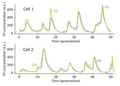
We chose the above traces because they showed the highest correlation between YFP and CFP levels. Other traces for lower expression levels have lower correlations due to effects of intrinsic noise (see Tables S2-S4). However, the existence of one trace in which YFP is almost perfectly proportional to CFP throughout can only occur if the YFP and CFP genes are under the same control. And, since the control of YFP and CFP genes in all of our synthetic circuits are identical (with the same promoters and plasmid positions), these data strongly suggest that our dual reporters are tightly co-regulated in all the synthetic circuits. Moreover, the negative control experiments presented in Fig. 3E provide a natural consistency check that the YFP and CFP are under the same control and satisfy Eq. (1).
We agree that it would be useful to know how much the X and Y production rates can differ for Eq. (2) to hold. Importantly, our proven theorem already allows for the rates to differ by an unspecified proportionality constant. In response to the referee’s comment we have derived a more general condition under which our approach holds. In the newly added SI Sec. 7 we prove that Eq. (2) holds also when rates differ as long as the difference is stochastic in nature with an average of zero. We also prove that Eq. (2) holds in the face of multiplicative noise that is independent of the X and Y production rates.
However, the production rates of X and Y cannot differ in all ways. Some types of differences between the X and Y production rates can lead to deviations of Eq. (2) even when there is no causal interaction. To highlight this, we added the results of simulations of a toy model in which the X and Y production rates differ by an additive noise term that does not average to zero, see Fig. S19B of the newly added SI Sec. 7.
- The invariant should potentially hold true for any biological species that are causally related e.g. protein-protein interactions. Also, this method could potentially find many applications in eukaryotic cells. Although it's outside the scope of current work to experimentally demonstrate such applications, the authors should comment on experimental strategies to apply this method to overcome potential pitfalls (e.g. presence of enhancers in eukaryotic cells).
We thank the referee for this suggestion. We agree that there are potential pitfalls that could come into effect when our proposed approach is applied on more complex systems such as eukaryotic gene expression. In response to the referee’s comment, we have added an explicit discussion of these potential pitfalls in the discussion section “Limitations of this study” (see p. 10).
In particular, in eukaryotes there are many genes in which promoter sequences may not be the sole factor determining transcription rates. Other factors that can be involved in gene regulation include the presence of enhancers, epigenetic modifications, and bursts in gene expression, to name a few. We thus propose a few strategies, which include positioning the passive reporter at a similar gene loci as the gene of interest, measuring the gene regulation activities of the gene of interest and its passive reporter using a separate method, and exploiting the invariant with a third gene, where it is known there is no causal interaction, as a consistency check. In addition, we include in the SI a new section SI Sec. 8 which shows that the invariant holds in the face of many types of bursty gene expression dynamics.
However, the above is not a comprehensive list. Some of the issues the referee mentions are serious and may not be straightforward to overcome. We now spell this out explicitly in the revised manuscript (p. 10).
- In the legend of Fig. 1, the sentence "Data points here are for..." is missing a few words, or needs to be rephrased.
We thank the referee for this comment. We have rewritten the figure caption, which now reads “Data points are numerical simulations of specific example networks (see SI for details) to illustrate the analytically proven theorem of Eq. 2.”
- Fig. 2 talks about the uncertainties associated with each point on the scatter plots. However, it is difficult to understand the quantification in such a plot. It would be great to have a plot quantifying the uncertainties in the invariant relation for the different topologies studied, specifically in order to understand if one topology is consistently deviating more from the x=y line than the other topologies studied here.
We thank the referee for this suggestion. In the supplement of the revised manuscript we have added supplemental Figs. S3, S4, and S5 to separately quantify the uncertainty of the difference processes plotted in Fig. 2 and have added a new section (SI Sec. 11) to discuss the processes simulated in Fig. 2 in more detail. In short, each simulated process generated less than ~5% of outliers when considering 95% confidence intervals (with the max percentage deviation being 5.01% for process 5, see Fig. S5). These outliers were then simulated over a larger number of simulations to reduce the sampling error, which resulted in 0% of outliers (see Sec. “Confidence intervals for finite sampling error” on Materials and Methods on p. 11). Some simulated processes generated larger percentage errors in the normalized covariances than others, but this is expected as different processes have different dynamics which will result in different degrees of sampling of the underlying distributions.
Note, that the invariant of Eq. 2 is analytically proven for all tested topologies as none of the topologies include a causal effect from X to Z. Any deviation of the numerical data from the straight line prediction of Eq. 2 (right column in Fig. 2C) is due to the finite sampling of a stochastic process to estimate the true covariance from the sampling covariance. Any given parameter set was simulated several times which allowed us to estimate the sampling error from differences in between repeated samples. In the additional SI figures we now quantify this error for the different topologies.
In addition to the above changes we want to highlight that the purpose of the simulations presented in Fig. (2) is not to prove our statements or explore the behavior of different topologies. The purpose of the data presented in the right column of Fig. 2C is to illustrate the theoretical invariant and act as a numerical sanity check of our analytically proven result. In contrast, the data in the left column of Fig 2C illustrates that the correlations do not satisfy an invariant like Eq. 2 which applies to covariances but not correlations.
- The legend for Fig. 3 seems to end abruptly. There likely needs to be more.
We thank the referee for catching this mistake. We have corrected the accidentally truncated figure caption of Fig. 3.
- There is a typo in equation (5.3) on page 23 of supplementary material, there should be x instead of y in the degradation equation of x.
We thank the referee for catching this mistake which has been corrected in the revised manuscript.
- In the supplemental material, to understand the unexpected novel discovery of causality, Figure S5 is presented. However, this doesn't give the context for other negative controls designed, and the effect of rfp dynamics (which can be seen in the plots both in the main paper and the supplement) in the growth rate of cells in those constructs. As a baseline, it would be nice to have those figures.
We thank the referee for this suggestion. We have now included representative RFP traces with the growth rates for other negative control circuits, see Fig. S10. In addition, we have now included the cross correlation functions between RFP and growth rate in these negative control circuits, see Fig. S10A. While in all cases, RFP and growth rate are negatively correlated, the outlier circuit exhibits the largest negative correlation.
The suggested comparison of the referee thus highlights that – in isolation – a negative correlation between RFP and growth rate is only weak evidence for our hypothesized causal interaction because negative correlations can result from the effect of growth rate affecting volume dilution and thus RFP concentration. Crucially, we thus additionally considered the overall variability of growth rate and found the outlier circuit has the largest growth rate variability which is indicative of something that is affecting the growth rate of those cells, see Fig. S10B. To compare the magnitude of RFP variability against other strains requires constraining the comparison group to other synthetic circuits that have RFP located on the chromosome rather than a plasmid. This is why we compare the CV of the outlier with the CV of circuit #5, which corresponds to the “regular” repressilator (i.e., the outlier circuit without the endogenous lacI gene). As an additional comparison, we computed the CV for a strain of E. coli that does not contain a synthetic plasmid at all, but still contains the RFP gene on the chromosome. We find that the CVs in the outlier circuit to be larger than in these two additional circuits, suggesting that the outlier circuit causes additional fluctuations in the RFP and growth rate. We now spell this out explicitly in the revised manuscript (see Sec. “Evidence that RpoS mediated stress response affected cellular growth in the outlier circuit“, p. 8).
The referee is correct that the above arguments are only circumstantial evidence, but they do show that the data is consistent with a plausible explanation of the hypothesized causal interaction. Our main evidence for an RpoS mediated stress response that explains the deviations from Eq. 2 in the outlier circuit is the perturbation experiment in which the deviation disappears for the RpoS knockout strain. We now spell out this argument explicitly in the revised manuscript (see Sec. “Evidence that RpoS mediated stress response affected cellular growth in the outlier circuit“, p. 8).
Reviewer #2 (Recommendations For The Authors):
The proof of theorem 1 relies on an earlier result, lemma 1. Lemma 1 only guarantees the existence of a "dummy" system that satisfies the separation requirement and preserves the dynamics of X and Y. However, in principle, it may be possible to maintain the dynamics of X and Y while still changing the relationship between Cov(X,Zk) and Cov(Y,Zk). This could occur if the dynamics of Zk differ in a particular way between the original system and the dummy system. So lemma 1 needs to be a little stronger- it needs to mention that the dynamics of Zk are preserved, or something along these lines. The proof of lemma 1 appears to contain the necessary ingredients for what is actually needed, but this should be clarified.
We agree with the referee that this is an important distinction. Lemma 1 does in fact guarantee that any component Zk that is not affected by X and Y will have the same dynamics in the “dummy” system. However, as the referee points out, this is not stated in the lemma statement nor in the proof of the lemma. In response to the referee’s comment, we have made it clear in the lemma statement that the Zk dynamics are preserved in the “dummy” system, and we have also added details to the proof to show that this is the case, see Lemma 1 on p. 27 of the SI.
Readers who are familiar with chemical reaction diagrams, but not birth-death process diagrams may waste some time trying to interpret Equation 1 as a chemical reaction diagram with some sort of rate constant as a label on each arrow (I did this). It may be helpful to either provide a self-contained definition of the notation used, or mention a source where the necessary definitions can be found.
We agree with the referee. In the revised manuscript we have added a description of the notation used below Equation 1 of the main text, see p. 2. The notational overloading of the “arrow notation” is a perennial problem in the field and we thank the referee for reminding us of the need to clarify what the arrows mean in our diagrams.
It would be helpful if the authors could propose a rule for deciding whether dependence is detected or not. As it stands presently, the output of the approach seems to be a chart like that in Figure 3D where you show eta_xz and eta_yz with confidence interval bars and the reader must visually assess whether the points more-or-less fall on the line of unity. It would be better to have some systematic procedure for making a "yes or no" call as to whether a causal link was detected or not. Having a systematic detection rule would allow you to make a call as to whether dependence in circuit 3 was detected or not. It would also allow you or a future effort to evaluate the true positive rate of the approach in simulated settings.
We thank the referee for this suggestion. In the revised manuscript we have added an explicit rule for detecting causality using the invariant of Eq. (2). Specifically, Eq. (2) can be re-written as r = 1 where r is the covariability ratio r = etaXZ/etaYZ. In that case, given 95% confidence intervals for the experimentally determined covariability ratio r, we say that there is a causal interaction if the confidence intervals overlap with the value of r = 1.
This corresponds to a null hypothesis test at the 2.5% significance level. The reason that it is at 2.5% significance and not 5% significance is as follows. Let’s say we measure a covariability ratio of r_m, and the 95% confidence interval is [r_m - e_m, r_m + e_m] for some error e_m. Without loss of generality, let’s say that r_m > 1 (the same applies if r_m < 1). This means that Prob(r < r_m - e_m) = 2.5% and Prob(r > r_m + e_m) = 2.5% , where r is the actual value of the covariability ratio. Under the null hypothesis that there is no causal interaction, we set r = 1. However, we now have Prob(1 < r_m + e_m) = 0, because we know that r_m > 1 and so we must have r_m + e_m > 1. The probability that the value of 1 falls outside the error bars is therefore 2.5% under the null hypothesis.
This proposed rule is the same rule that we used to detect statistical outliers in our simulations, where we found a “false positive” rate of 2.3% over 6522 simulated systems due to statistical sampling error (as discussed in the Materials and Methods section). In response to the referee’s suggestion, we have added the section “A rule for detecting causality in the face of measurement uncertainty” (p. 4). We also apply the rule to the experimental data and find that the rule detects 2/4 causal interactions in Fig. 3D. We have clarified this in the Fig. 3D caption, in the main text, and we have added a figure in the SI (Fig. S2) where we apply the null hypothesis test on the measured covariability ratios.
Note, whether the third interaction is “detected” or not depends on the cut-off value used. We picked the most common 95% rule to be consistent with the traditional statistical approaches. With this rule one of the data points lies right at the cusp of detection, but ultimately falls into the “undetected” category if a strictly binary answer is sought under the above rule.
It would be helpful to mention what happens when the abundance of a species hits zero. Specifically, there are two ways to interpret the arrow from X to X+d with a W on top:
Interpretation (1):
P(X+d | X) = W if X+d {greater than or equal to} 0 P(X+d | X) = 0 if X_i+d_i < 0 for at least one i
Interpretation (2):
P(X+d | X) = W regardless of whether X+d < 0 W = 0 whenever X_i < d_i for at least one i
Interpretation (1) corresponds to a graph where the states are indexed on the non-negative integers. Interpretation (2) corresponds to a graph where the states are indexed on the integers (positive or negative), and W is responsible for enforcing the non-negativity of mass. I believe you need the second interpretation because the first interpretation leads to problems with your definition of causality. For example, consider the reaction:
(Na, K) -- 0.1 --> (Na-1, K+1)
This could occur if Na and K are the intracellular concentrations of sodium and potassium ions in a cell that has an ATP-driven sodium-potassium exchanger whose rate is limited by the frequency with which extracellular potassium ions happen to flow by. Per the definition of causality found in the appendix, Na has no causal effect on K since Na does not show up in the reaction rate term. However, under interpretation (1), Na clearly has a causal effect on K according to a reasonable definition of causality because if Na=0, then the reaction cannot proceed, whereas if Na>0 then it can. However, under interpretation (2), the reaction above cannot exist and so this scenario is excluded.
We thank the referee for this comment that helped us clarify the meaning of arrows with propensities. In short, interpretation (2) corresponds to the definition of our stochastic systems. This is consistent with the standard notation used for the chemical master equation. As the referee points out, because molecular abundances cannot be negative, any biochemical system must then have the property that the propensity of a reaction must be equal to zero when the system is in a state in which an occurrence of that reaction would take one of the abundances to negative numbers. Stochastic networks that do not have this property cannot correspond to biochemical reaction networks.
In the revised manuscript, we now spell this out explicitly to avoid any confusion, see SI page 25.
Furthermore, we additionally discuss the referee’s example in which the rate of exchanging Na for K through an ion exchanger is approximately independent of the intracellular Na concentration. Because biochemical systems cannot become negative, it cannot be that the rate is truly constant, but at some point for low concentrations must go down until it becomes exactly zero for zero molecules.
Importantly, agreement with Eq. (2) does not imply that there is no causal effect from X to Zk. It is the deviation from Eq. (2) that implies the existence of a causal effect from X to Zk. Therefore, although the above referee’s example would constitute a causal interaction in our framework, it would not lead to a deviation of Eq. (2) because the fluctuations in Na (which we exploit) do not propagate to K. From a practical point of view, our method thus detects whether changing X over the observed range affects the production and degradation rates of Zk.
In the course of setting up the negative control benchmark circuits, a perturbation-based causal validation would be nice. For instance, first, verify that X does not affect Z by intervening on X (e.g. changing its copy number or putting it under the control of an inducible promoter), and ensuring that Z's activity is not affected by such interventions upon X. This approach would help to adjudicate questions of whether the negative control circuits actually have an unknown causal link. The existing benchmark is already reasonably solid in my view, and I do not know how feasible this would be with the authors' setup, but I think that a perturbation-based validation could in principle be the gold standard benchmark.
We agree that additional perturbation-based validation tests on all of the negative control circuits would indeed improve the evidence that our method worked as advertised. While such experiments are indeed beyond the scope of our current work we now explicitly point out the benefits of such additional controls in the revised Discussion.
Below is a series of comments about typography, mostly about section 4 of the supplement.
We thank the referee for their careful reading and highlighting those mistakes.
At the bottom of page 21, Z_aff is defined as the set of components that are affected by X. However, later Z_aff seems to refer to components affected by X or Y. For instance, in the proof of lemma 1, it is written "However, because a is part of z_aff, the {ak} variables must be affected by X and/or Y."
We thank the referee for catching this mistake. We have changed the definition of Z_aff throughout the supplement to refer to components affected by X or Y. If it can be experimentally ensured that Y is a passive reporter (i.e., it does not affect other components in the cell), then the theorem can only be violated if X affects Z.
In the equation following Eq 5.2, W_k and d_k should be W_i and d_i ?
Yes, the referee is correct. In the revised manuscript we have corrected W_k and d_k to W_i and d_i.
In Eq 5.3 in the lower-left transition diagram, I think a "y" should be an "x".
Yes, the referee is correct. In the revised manuscript we have fixed this typo.
In the master equation above Eq 5.5, the "R" terms for the y reactions are missing the alpha term, and I think two of the beta terms need to be multiplied by x and y respectively.
The referee is correct. In the revised manuscript we have fixed this typo.
The notation of Eq 5.8, where z_k(t) is the conditional expectation of z_kt, is strange and difficult to follow. Why does z_k(t) not get a bar over it like its counterparts for x, y, R, and beta? The bars, although not a perfect solution, do help.
We agree with the referee’s comment and have added further explanations to define the averages in question, see SI p. 28. In short, when we condition on the history of the components not affected by X or Y, we in effect condition on the time trajectories of z_{k} (when it is part of the components not affected by X and/or Y) and beta (since it only depends on the components not affected by X or Y). We thus previously did not include the bars when taking the averages of these components in the conditional space because the conditioning in effect sets their time-trajectories (so they become deterministic functions of time). In the revised manuscript we now also denote these conditional expectations with bars and we have added comments to the proof to clarify their definition.
I think it would be helpful to show how the relationship =/alpha is obtained from Eq 5.5.
We agree with this suggestion and have added the derivations, see Eqs. (5.9) - (5.13) in the revised SI.
In the main text, the legend of Fig 3 cuts off mid-sentence.
We thank the referee for catching this mistake which has been fixed in the revised manuscript.
-
-
eLife assessment
By taking advantage of noise in gene expression, this important study introduces a new approach for detecting directed causal interactions between two genes without perturbing either. The main theoretical result is supported by a proof, although clearer statements are needed to ensure that there are no edge cases that can violate the theorem. Preliminary simulations and experiments on small circuits are presented, but the evidence remains incomplete because further investigations are needed to demonstrate the broad applicability and scalability of the method.
-
Reviewer #1 (Public Review):
Summary:
This manuscript presents a method to infer causality between two genes (and potentially proteins or other molecules) based on the non-genetic fluctuations among cells using a version of the dual-reporter assay as a causal control, where one half of the dual-reporter pair is causally decoupled, as it is inactive. The authors propose a statistical invariant identity to formalize this idea.Strengths:
The paper outlines a theoretical formalism, which, if experimentally used, can be useful in causal network inference, which is a great need in the study of biological systems.Weaknesses:
The practical utility of this method may not be straightforward and potentially be quite difficult to execute. Additionally, further investigations are needed to provide evidence of the broad applicability of the method …Reviewer #1 (Public Review):
Summary:
This manuscript presents a method to infer causality between two genes (and potentially proteins or other molecules) based on the non-genetic fluctuations among cells using a version of the dual-reporter assay as a causal control, where one half of the dual-reporter pair is causally decoupled, as it is inactive. The authors propose a statistical invariant identity to formalize this idea.Strengths:
The paper outlines a theoretical formalism, which, if experimentally used, can be useful in causal network inference, which is a great need in the study of biological systems.Weaknesses:
The practical utility of this method may not be straightforward and potentially be quite difficult to execute. Additionally, further investigations are needed to provide evidence of the broad applicability of the method to naturally occurring systems and its scalability beyond the simple circuit in which it is experimentally demonstrated. -
Reviewer #2 (Public Review):
Summary:
This paper describes a new approach to detecting directed causal interactions between two genes without directly perturbing either gene. To check whether gene X influences gene Z, a reporter gene (Y) is engineered into the cell in such a way that (1) Y is under the same transcriptional control as X, and (2) Y does not influence Z. Then, under the null hypothesis that X does not affect Z, the authors derive an equation that describes the relationship between the covariance of X and Z and the covariance of Y and Z. Violation of this relationship can then be used to detect causality.The authors benchmark their approach experimentally in several synthetic circuits. In four positive control circuits, X is a TetR-YFP fusion protein that represses Z, which is an RFP reporter. The proposed approach …
Reviewer #2 (Public Review):
Summary:
This paper describes a new approach to detecting directed causal interactions between two genes without directly perturbing either gene. To check whether gene X influences gene Z, a reporter gene (Y) is engineered into the cell in such a way that (1) Y is under the same transcriptional control as X, and (2) Y does not influence Z. Then, under the null hypothesis that X does not affect Z, the authors derive an equation that describes the relationship between the covariance of X and Z and the covariance of Y and Z. Violation of this relationship can then be used to detect causality.The authors benchmark their approach experimentally in several synthetic circuits. In four positive control circuits, X is a TetR-YFP fusion protein that represses Z, which is an RFP reporter. The proposed approach detected the repression interaction in two or three of the positive control circuits. The authors constructed sixteen negative control circuit designs in which X was again TetR-YFP, but where Z was either a constitutively expressed reporter or simply the cellular growth rate. The proposed method detected a causal effect in two of the sixteen negative controls, which the authors argue is not a false positive, but due to an unexpected causal effect. Overall, these pilot studies, albeit in simplified scenarios, provide encouraging results.
Strengths:
The idea of a "no-causality control" in the context of detected directed gene interactions is a valuable conceptual advance that could potentially see play in a variety of settings where perturbation-based causality detection experiments are made difficult by practical considerations.By proving their mathematical result in the context of a continuous-time Markov chain, the authors use a more realistic model of the cell than, for instance, a set of deterministic ordinary differential equations.
Caveats:
The term "causally" is used in the main-text statement of the central theorem (Eq 2) without a definition of this term. This makes it difficult to fully understand the statement of the paper's central theorem without diving into the supplement.The basic argument of theorem 1 appears to rely on establishing that x(t) and y(t) are independent of their initial conditions. Yet, there appear to be some scenarios where this property breaks down:
(1) Theorem 1 does not seem to hold in the edge case where R=beta=W=0, meaning that the components of interest do not vary with time, or perhaps vary in time only due to measurement noise. In this case x(t), y(t), and z(t) depend on x(0), y(0), and z(0). Since the distributions of x(0), y(0), and z(0) are unspecified, a counterexample to the theorem may be readily constructed by manipulating the covariance matrix of x(0), y(0), and z(0).
(2) A similar problem may occur when transition probabilities decay with time. For example, suppose that again R=0 and X are degraded by a protease (B), but this protease is subject to its own first-order degradation. The deterministic version of this situation can be written, for example, dx/dt=-bx and db/dt=-b. In this system, x(t) approaches x(0)exp(-b(0)) for large t. Thus, as above, x(t) depends on x(0). If similar dynamics apply to the Y and Z genes, we can make all genes depend on their initial conditions, thus producing a pathology analogous to the above example.
The reviewer does not know when such examples may occur in (bio)physical systems. Nevertheless, since one of the advantages of mathematics is the ability to correctly identify the domain of validity for a claim, the present work would be strengthened by "building a fence" around these edge cases, either by identifying the comprehensive set of such edge cases and explicitly prohibiting them in a stated assumption set, or by pointing out how the existing assumptions already exclude them.
-
