Motor cortex activity across movement speeds is predicted by network-level strategies for generating muscle activity
Curation statements for this article:-
Curated by eLife

Evaluation Summary:
This study investigates the mechanisms by which distributed systems control rhythmic movements of different speeds. The authors train an artificial recurrent neural network to produce the muscle activity patterns that monkeys generate when performing an arm cycling task at different speeds. The dominant patterns in the neural network do not directly reflect muscle activity and these dominant patterns do a better job than muscle activity at capturing key features of neural activity recorded from the monkey motor cortex in the same task. The manuscript is easy to read and the data and modelling are intriguing and well done. Further work should better explain some of the neural network assumptions and how these assumptions relate to the treatment of the empirical data and its interpretation.
(This preprint has been reviewed by eLife. We include the public reviews from the reviewers here; the authors also receive private feedback with suggested changes to the manuscript. The reviewers remained anonymous to the authors.)
This article has been Reviewed by the following groups
Discuss this preprint
Start a discussion What are Sciety discussions?Listed in
- Evaluated articles (eLife)
Abstract
Learned movements can be skillfully performed at different paces. What neural strategies produce this flexibility? Can they be predicted and understood by network modeling? We trained monkeys to perform a cycling task at different speeds, and trained artificial recurrent networks to generate the empirical muscle-activity patterns. Network solutions reflected the principle that smooth well-behaved dynamics require low trajectory tangling. Network solutions had a consistent form, which yielded quantitative and qualitative predictions. To evaluate predictions, we analyzed motor cortex activity recorded during the same task. Responses supported the hypothesis that the dominant neural signals reflect not muscle activity, but network-level strategies for generating muscle activity. Single-neuron responses were better accounted for by network activity than by muscle activity. Similarly, neural population trajectories shared their organization not with muscle trajectories, but with network solutions. Thus, cortical activity could be understood based on the need to generate muscle activity via dynamics that allow smooth, robust control over movement speed.
Article activity feed
-

-

Author Response:
Evaluation Summary:
This study investigates the mechanisms by which distributed systems control rhythmic movements of different speeds. The authors train an artificial recurrent neural network to produce the muscle activity patterns that monkeys generate when performing an arm cycling task at different speeds. The dominant patterns in the neural network do not directly reflect muscle activity and these dominant patterns do a better job than muscle activity at capturing key features of neural activity recorded from the monkey motor cortex in the same task. The manuscript is easy to read and the data and modelling are intriguing and well done.
We thank the editor and reviewers for this accurate summary and for the kind words.
Further work should better explain some of the neural network assumptions and how these …
Author Response:
Evaluation Summary:
This study investigates the mechanisms by which distributed systems control rhythmic movements of different speeds. The authors train an artificial recurrent neural network to produce the muscle activity patterns that monkeys generate when performing an arm cycling task at different speeds. The dominant patterns in the neural network do not directly reflect muscle activity and these dominant patterns do a better job than muscle activity at capturing key features of neural activity recorded from the monkey motor cortex in the same task. The manuscript is easy to read and the data and modelling are intriguing and well done.
We thank the editor and reviewers for this accurate summary and for the kind words.
Further work should better explain some of the neural network assumptions and how these assumptions relate to the treatment of the empirical data and its interpretation.
The manuscript has been revised along these lines.
Reviewer #1 (Public Review):
In this manuscript, Saxena, Russo et al. study the principles through which networks of interacting elements control rhythmic movements of different speeds. Typically, changes in speed cannot be achieved by temporally compressing or extending a fixed pattern of muscle activation, but require a complex pattern of changes in amplitude, phase, and duty cycle across many muscles. The authors train an artificial recurrent neural network (RNN) to predict muscle activity measured in monkeys performing an arm cycling task at different speeds. The dominant patterns of activity in the network do not directly reflect muscle activity. Instead, these patterns are smooth, elliptical, and robust to noise, and they shift continuously with speed. The authors then ask whether neural population activity recorded in motor cortex during the cycling task closely resembles muscle activity, or instead captures key features of the low-dimensional RNN dynamics. Firing rates of individual cortical neurons are better predicted by RNN than by muscle activity, and at the population level, cortical activity recapitulates the structure observed in the RNN: smooth ellipses that shift continuously with speed. The authors conclude that this common dynamical structure observed in the RNN and motor cortex may reflect a general solution to the problem of adjusting the speed of a complex rhythmic pattern. This study provides a compelling use of artificial networks to generate a hypothesis on neural population dynamics, then tests the hypothesis using neurophysiological data and modern analysis methods. The experiments are of high quality, the results are explained clearly, the conclusions are justified by the data, and the discussion is nuanced and helpful. I have several suggestions for improving the manuscript, described below.
This is a thorough and accurate summary, and we appreciate the kind comments.
It would be useful for the authors to elaborate further on the implications of the study for motor cortical function. For example, do the authors interpret the results as evidence that motor cortex acts more like a central pattern generator - that is, a neural circuit that transforms constant input into rhythmic output - and less like a low-level controller in this task?
This is a great question. We certainly suspect that motor cortex participates in all three key components: rhythm generation, pattern generation, and feedback control. The revised manuscript clarifies how the simulated networks perform both rhythm generation and muscle-pattern generation using different dimensions (see response to Essential Revisions 1a). Thus, the stacked-elliptical solution is consistent with a solution that performs both of these key functions.
We are less able to experimentally probe the topic of feedback control (we did not deliver perturbations), but agree it is important. We have thus included new simulations in which networks receive (predictable) sensory feedback. These illustrate that the stacked-elliptical solution is certainly compatible with feedback impacting the dynamics. We also now discuss that the stacked-elliptical structure is likely compatible with the need for flexible responses to unpredictable perturbations / errors:
"We did not attempt to simulate feedback control that takes into account unpredictable sensory inputs and produces appropriate corrections (Stavisky et al. 2017; Pruszynski and Scott 2012; Pruszynski et al. 2011; Pruszynski, Omrani, and Scott 2014). However, there is no conflict between the need for such control and the general form of the solution observed in both networks and cortex. Consider an arbitrary feedback control policy: 𝑧 = 𝑔 𝑐 (𝑡, 𝑢 𝑓 ) where 𝑢 is time-varying sensory input arriving in cortex and is a vector of outgoing commands. The networks we 𝑓 𝑧 trained all embody special cases of the control policy where 𝑢 is either zero (most simulations) or predictable (Figure 𝑓
- and the particulars of 𝑧 vary with monkey and cycling direction. The stacked-elliptical structure was appropriate in all these cases. Stacked-elliptical structure would likely continue to be an appropriate scaffolding for control policies with greater realism, although this remains to be explored."
The observation that cortical activity looks more like the pattern-generating modes in the RNN than the EMG seem to be consistent with this interpretation. On the other hand, speed-dependent shifts for motor cortical activity in walking cats (where the pattern generator survives the removal of cortex and is known to be spinal) seems qualitatively similar to the speed modulation reported here, at least at the level of single neurons (e.g., Armstrong & Drew, J. Physiol. 1984; Beloozerova & Sirota, J. Physiol. 1993). More generally, the authors may wish to contextualize their work within the broader literature on mammalian central pattern generators.
We agree our discussion of this topic was thin. We have expanded the relevant section of the Discussion. Interestingly, Armstrong 1984 and Beloozerova 1993 both report quite modest changes in cortical activity with speed during locomotion (very modest in the case of Armstrong). The Foster et al. study agrees with those earlier studies, although the result is more implicit (things are stacked, but separation is quite small). Thus, there does seem to be an intriguing difference between what is observed in cortex during cycling (where cortex presumably participates heavily in rhythm/pattern generation) and during locomotion (where it likely does not, and concerns itself more with alterations of gait). This is now discussed:
"Such considerations may explain why (Foster et al. 2014), studying cortical activity during locomotion at different speeds, observed stacked-elliptical structure with far less trajectory separation; the ‘stacking’ axis captured <1% of the population variance, which is unlikely to provide enough separation to minimize tangling. This agrees with the finding that speed-based modulation of motor cortex activity during locomotion is minimal (Armstrong and Drew 1984) or modest (Beloozerova and Sirota 1993). The difference between cycling and locomotion may reflect cortex playing a less-central role in the latter. Cortex is very active during locomotion, but that may reflect cortex being ‘informed’ of the spinally generated locomotor rhythm for the purpose of generating gait corrections if necessary (Drew and Marigold 2015; Beloozerova and Sirota 1993). If so, there would be no need for trajectories to be offset between speeds because they are input-driven, and need not display low tangling."
For instance, some conclusions of this study seem to parallel experimental work on the locomotor CPG, where a constant input (electrical or optogenetic stimulation of the MLR at a frequency well above the stepping rate) drives walking, and changes in this input smoothly modulate step frequency.
We now mention this briefly when introducing the simulated networks and the modeling choices that we made:
"Speed was instructed by the magnitude of a simple static input. This choice was made both for simplicity and by rough analogy to the locomotor system; spinal pattern generation can be modulated by constant inputs from supraspinal areas (Grillner, S. 1997). Of course, cycling is very unlike locomotion and little is known regarding the source or nature of the commanding inputs. We thus explore other possible input choices below."
If the input to the RNN were rhythmic, the network dynamics would likely be qualitatively different. The use of a constant input is reasonable, but it would be useful for the authors to elaborate on this choice and its implications for network dynamics and control. For example, one might expect high tangling to present less of a problem for a periodically forced system than a time-invariant system. This issue is raised in line 210ff, but could be developed a bit further.
To investigate, we trained networks (many, each with a different initial weight initialization) to perform the same task but with a periodic forcing input. The stacked-elliptical solution often occurred, but other solutions were also common. The non-stacking solutions relied strongly on the ‘tilt’ strategy, where trajectories tilt into different dimensions as speed changes. There is of course nothing wrong with the ‘tilting’ strategy; it is a perfectly good way to keep tangling low. And of course it was also used (in addition to stacking) by both the empirical data and by graded-input networks (see section titled ‘Trajectories separate into different dimensions’). This is now described in the text (and shown in Figure 3 - figure supplement 2):
"We also explored another plausible input type: simple rhythmic commands (two sinusoids in quadrature) to which networks had to phase-lock their output. Clear orderly stacking with speed was prominent in some networks but not others (Figure 3 - figure supplement 2a,b). A likely reason for the variability of solutions is that rhythmic-input-receiving networks had at least two “choices”. First, they could use the same stacked-elliptical solution, and simply phase-lock that solution to their inputs. Second, they could adopt solutions with less-prominent stacking (e.g., they could rely primarily on ‘tilting’ into new dimensions, a strategy we discuss further in a subsequent section)."
This addition is clarifying because knowing that there are other reasonable solutions (e.g., pure tilt with little stacking), as it makes it more interesting that the stacked-elliptical solution was observed empirically. At the same time, the lesson to be drawn from the periodically forced networks isn’t 100% clear. They sometimes produced solutions with realistic stacking, so they are clearly compatible with the data. On the other hand, they didn’t do so consistently, so perhaps this makes them a bit less appealing as a hypothesis. Potentially more appealing is the hypothesis that both input types (a static, graded input instructing speed and periodic inputs instructing phase) are used. We strongly suspect this could produce consistently realistic solutions. However, in the end we decided we didn’t want to delve too much into this, because neither our data nor our models can strongly constrain the space of likely network inputs. This is noted in the Discussion:
"The desirability of low tangling holds across a broad range of situations (Russo et al. 2018). Consistent with this, we observed stacked-elliptical structure in networks that received only static commands, and in many of the networks that received rhythmic forcing inputs. Thus, the empirical population response is consistent with motor cortex receiving a variety of possible input commands from higher motor areas: a graded speed-specifying command, phase-instructing rhythmic commands, or both.."
The use of a constant input should also be discussed in the context of cortical physiology, as motor cortex will receive rhythmic (e.g., sensory) input during the task. The argument that time-varying input to cortex will itself be driven by cortical output (475ff) is plausible, but the underlying assumption that cortex is the principal controller for this movement should be spelled out. Furthermore, this argument would suggest that the RNN dynamics might reflect, in part, the dynamics of the arm itself, in addition to those of the brain regions discussed in line 462ff. This could be unpacked a bit in the Discussion.
We agree this is an important topic and worthy of greater discussion. We have also added simulations that directly address this topic. These are shown in the new Figure 9 and described in the new section ‘Generality of the network solution’:
"Given that stacked-elliptical structure can instantiate a wide variety of input-output relationships, a reasonable question is whether networks continue to adopt the stacked-elliptical solution if, like motor cortex, they receive continuously evolving sensory feedback. We found that they did. Networks exhibited the stacked-elliptical structure for a variety of forms of feedback (Figure 9b,c, top rows), consistent with prior results (Sussillo et al. 2015). This relates to the observation that “expected” sensory feedback (i.e., feedback that is consistent across trials) simply becomes part of the overall network dynamics (M. G. Perich et al. 2020). Network solutions remained realistic so long as feedback was not so strong that it dominated network activity. If feedback was too strong (Figure 9b,c, bottom rows), network activity effectively became a representation of sensory variables and was no longer realistic."
We agree that the observed dynamics may “reflect, in part, the dynamics of the arm itself, in addition to those of the brain regions discussed”, as the reviewer says. At the same time, it seems to us quite unlikely that they primarily reflect the dynamics of the arm. We have added the following to the Discussion to outline what we think is most likely:
"This second observation highlights an important subtlety. The dynamics shaping motor cortex population trajectories are widely presumed to reflect multiple forms of recurrence (Churchland et al. 2012): intracortical, multi-area (Middleton and Strick 2000; Wang et al. 2018; Guo et al. 2017; Sauerbrei et al. 2020) and sensory reafference (Lillicrap and Scott 2013; Pruszynski and Scott 2012). Both conceptually (M. G. Perich et al. 2020) and in network models (Sussillo et al. 2015), predictable sensory feedback becomes one component supporting the overall dynamics. Taken to an extreme, this might suggest that sensory feedback is the primary source of dynamics. Perhaps what appear to be “neural dynamics” merely reflect incoming sensory feedback mixed with outgoing commands. A purely feedforward network could convert the former into the latter, and might appear to have rich dynamics simply because the arm does (Kalidindi et al. 2021). While plausible, this hypothesis strikes us as unlikely. It requires sensory feedback, on its own, to create low-tangled solutions across a broad range of tasks. Yet there exists no established property of sensory signals that can be counted on to do so. If anything the opposite is true: trajectory tangling during cycling is relatively high in somatosensory cortex even at a single speed (Russo et al. 2018). The hypothesis of purely sensory-feedback-based dynamics is also unlikely because population dynamics begin unfolding well before movement begins (Churchland et al. 2012). To us, the most likely possibility is that internal neural recurrence (intra- and inter-area) is adjusted during learning to ensure that the overall dynamics (which will incorporate sensory feedback) provide good low-tangled solutions for each task. This would mirror what we observed in networks: sensory feedback influenced dynamics but did not create its dominant structure. Instead, the stacked-elliptical solution emerged because it was a ‘good’ solution that optimization found by shaping recurrent connectivity."
As the reviewer says, our interpretation does indeed assume M1 is central to movement control. But of course this needn’t (and probably doesn’t) imply dynamics are only due to intra-M1 recurrence. What is necessarily assumed by our perspective is that M1 is central enough that most of the key signals are reflected there. If that is true, tangling should be low in M1. To clarify this reasoning, we have restructured the section of the Discussion that begins with ‘Even when low tangling is desirable’.
The low tangling in the dominant dimensions of the RNN is interpreted as a signature of robust pattern generation in these dimensions (lines 207ff, 291). Presumably, dimensions related to muscle activity have higher tangling. If these muscle-related dimensions transform the smooth, rhythmic pattern into muscle activity, but are not involved in the generation of this smooth pattern, one might expect that recurrent dynamics are weaker in these muscle-related dimensions than in the first three principal components. That is, changes along the dominant, pattern-generating dimensions might have a strong influence on muscle-related dimensions, while changes along muscle-related dimensions have little impact on the dominant dimensions. Is this the case?
A great question and indeed it is the case. We have added perturbation analyses of the model showing this (Figure 3f). The results are very clear and exactly as the reviewer intuited.
It would be useful to have more information on the global dynamics of the RNN; from the figures, it is difficult to determine the flow in principal component space far from the limit cycle. In Fig. 3E (right), perturbations are small (around half the distance to the limit cycle for the next speed); if the speed is set to eight, would trajectories initialized near the bottom of the panel converge to the red limit cycle? Visualization of the vector field on a grid covering the full plotting region in Fig. 3D-E with different speeds in different subpanels would provide a strong intuition for the global dynamics and how they change with speed.
We agree that both panels in Figure 3e were hard to visually parse. We have improved it, but fundamentally it is a two-dimensional projection of a flow-field that exists in many dimensions. It is thus inevitable that it is hard to follow the details of the flow-field, and we accept that. What is clear is that the system is stable: none of the perturbations cause the population state to depart in some odd direction, or fall into some other attractor or limit cycle. This is the main point of this panel and the text has been revised to clarify this point:
"When the network state was initialized off a cycle, the network trajectory converged to that cycle. For example, in Figure 3e (left) perturbations never caused the trajectory to depart in some new direction or fall into some other limit cycle; each blue trajectory traces the return to the stable limit cycle (black).
Network input determined which limit cycle was stable (Figure 3e, right)."
One could of course try and determine more about the flow-fields local to the trajectories. E.g., how quickly do they return activity to the stable orbit? We now explore some aspects of this in the new Figure 3f, which gets at a property that is fundamental to the elliptical solution. At the same time, we stress that some other details will be network specific. For example, networks trained in the presence of noise will likely have a stronger ‘pull’ back to the canonical trajectory. We wish to avoid most of these details to allow us to concentrate on features of the solution that
- were preserved across networks and 2) could be compared with data.
What was the goodness-of-fit of the RNN model for individual muscles, and how was the mean-squared error for the EMG principal components normalized (line 138)? It would be useful to see predicted muscle activity in a similar format as the observed activity (Fig. 2D-F), ideally over two or three consecutive movement cycles.
The revision clarifies that the normalization is just the usual one we are all used to when computing the R^2 (normalization by total variance). We have improved this paragraph:
"Success was defined as <0.01 normalized mean-squared error between outputs and targets (i.e., an R^2 > 0.99). Because 6 PCs captured ~95% of the total variance in the muscle population (94.6 and 94.8% for monkey C and D), linear readouts of network activity yielded the activity of all recorded muscles with high fidelity."
Given this accuracy, plotting network outputs would be redundant with plotting muscle activity as they would look nearly identical (and small differences would of course be different for every network.
A related issue is whether the solutions are periodic for each individual node in the 50-dimensional network at each speed (as is the case for the first few RNN principal components and activity in individual cortical neurons and the muscles). If so, this would seem to guarantee that muscle decoding performance does not degrade over many movement cycles. Some additional plots or analysis might be helpful on this point: for example, a heatmap of all dimensions of v(t) for several consecutive cycles at the same speed, and recurrence plots for all nodes. Finally, does the period of the limit cycle in the dominant dimensions match the corresponding movement duration for each speed?
These are good questions; it is indeed possible to obtain ‘degenerate’ non-periodic solutions if one is not careful during training. For example, if during training, you always ask for 3 cycles, it becomes possible for the network to produce a periodic output based on non-periodic internal activity. To ensure this did not happen, we trained networks with variable number of cycles. Inspection confirmed this was successful: all neurons (and the ellipse that summarizes their activity) showed periodic activity. These points are now made in the text:
"Networks were trained across many simulated “trials”, each of which had an unpredictable number of cycles. This discouraged non-periodic solutions, which would be likely if the number of cycles were fixed and small.
Elliptical network trajectories formed stable limit cycles with a period matching that of the muscle activity at each speed."
We also revised the relevant section of the Methods to clarify how we avoided degenerate solutions, see section beginning with:
“One concern, during training, is that networks may learn overly specific solutions if the number of cycles is small and stereotyped”.
How does the network respond to continuous changes in input, particularly near zero? If a constant input of 0 is followed by a slowly ramping input from 0-1, does the solution look like a spring, as might be expected based on the individual solutions for each speed? Ramping inputs are mentioned in the Results (line 226) and Methods (line 805), but I was unable to find this in the figures. Does the network have a stable fixed point when the input is zero?
For ramping inputs within the trained range, it is exactly as the reviewer suggests. The figure below shows a slowly ramping input (over many seconds) and the resulting network trajectory. That trajectory traces a spiral (black) that traverses the ‘static’ solutions (colored orbits).
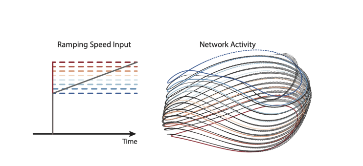
It is also true that activity returns to baseline levels when the input is turned off and network output ceases. For example, the input becomes zero at time zero in the plot below.
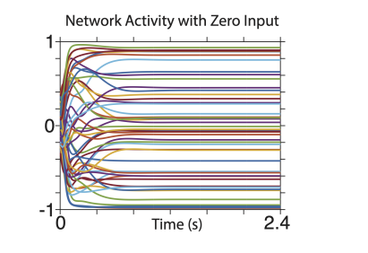
The text now notes the stability when stopping:
"When the input was returned to zero, the elliptical trajectory was no longer stable; the state returned close to baseline (not shown) and network output ceased."
The text related to the ability to alter speed ‘on the fly’ has also been expanded:
"Similarly, a ramping input produced trajectories that steadily shifted, and steadily increased in speed, as the input ramped (not shown). Thus, networks could adjust their speed anywhere within the trained range, and could even do so on the fly."
The Discussion now notes that this ramping of speed results in a helical structure. The Discussion also now notes, informally, that we have observed this helical structure in motor cortex. However, we don’t want to delve into that topic further (e.g., with direct comparisons) as those are different data from a different animal, performing a somewhat different task (point-to-point cycling).
As one might expect, network performance outside the trained range of speeds (e.g., during an input is between zero and the slowest trained speed) is likely to be unpredictable and network-specific. There is likely is a ‘minimum speed’ below which networks can’t cycle. This appeared to also be true of the monkeys; below ~0.5 Hz their cycling became non-smooth and they tended to stop at the bottom. (This is why our minimum speed is 0.8 Hz). However, it is very unclear whether there in any connection between these phenomena and we thus avoid speculating.
Why were separate networks trained for forward and backward rotations? Is it possible to train a network on movements in both directions with inputs of {-8, …, 8} representing angular velocity? If not, the authors should discuss this limitation and its implications.
Yes, networks can readily be trained to perform movements in both directions, each at a range of speeds. This is now stated:
"Each network was trained to produce muscle activity for one cycling direction. Networks could readily be trained to produce muscle activity for both cycling directions by providing separate forward- and backward-commanding inputs (each structured as in Figure 3a). This simply yielded separate solutions for forward and backward, each similar to that seen when training only that direction. For simplicity, and because all analyses of data involve within-direction comparisons, we thus consider networks trained to produce muscle activity for one direction at a time."
As noted, networks simply found independent solutions for forward and backward. This is consistent with prior work where the angle between forward and backward trajectories in state space is sizable (Russo et al. 2018) and sometimes approaches orthogonality (Schroeder et al. 2022).
It is somewhat difficult to assess the stability of the limit cycle and speed of convergence from the plots in Fig. 3E. A plot of the data in this figure as a time series, with sweeps from different initial conditions overlaid (and offset in time so trajectories are aligned once they're near the limit cycle), would aid visualization. Ideally, initial conditions much farther from the limit cycle (especially in the vertical direction) would be used, though this might require "cutting and pasting" the x-axis if convergence is slow. It might also be useful to know the eigenvalues of the linearized Poincaré map (choosing a specific phase of the movement) at the fixed point, if this is computationally feasible.
See response to comment 4 above. The new figure 3f now shows, as a time series, the return to the stable orbit after two types of perturbations. This specific analysis was suggested by the reviewer above, and we really like it because it gets at how the solution works. One could of course go further and try to ascertain other aspects of stability. However, we want to caution that is a tricky and uncertain path. We found that the overall stacked-elliptical solution was remarkably consistent among networks (it was shown by all networks that received a graded speed-specifying input). The properties documented in Figure 3f are a consistent part of that consistent solution. However, other detailed properties of the flow field likely won’t be. For example, some networks were trained in the presence of noise, and likely have a much more rapid return to the limit cycle. We thus want to avoid getting too much into those specifics, as we have no way to compare with data and determine which solutions mimic that of the brain.
Reviewer #2 (Public Review):
The study from Saxena et al "Motor cortex activity across movement speeds is predicted by network-level strategies for generating muscle activity" expands on an exciting set of observations about neural population dynamics in monkey motor cortex during well trained, cyclical arm movements. Their key findings are that as movement speed varies, population dynamics maintain detangled trajectories through stacked ellipses in state space. The neural observations resemble those generated by in silico RNNs trained to generate muscle activity patterns measured during the same cycling movements produced by the monkeys, suggesting a population mechanism for maintaining continuity of movement across speeds. The manuscript was a pleasure to read and the data convincing and intriguing. I note below ideas on how I thought the study could be improved by better articulating assumptions behind interpretations, defense of the novelty, and implications could be improved, noting that the study is already strong and will be of general interest.
We thank the reviewer for the kind words and nice summary of our results.
Primary concerns/suggestions:
1 Novelty: Several of the observations seem an incremental change from previously published conclusions. First, detangled neural trajectories and tangled muscle trajectories was a key conclusion of a previous study from Russo et al 2018. The current study emphasizes the same point with the minor addition of speed variance. Better argument of the novelty of the present conclusions is warranted. Second, the observations that motor cortical activity is heterogenous are not new. That single neuronal activity in motor cortex is well accounted for in RNNs as opposed to muscle-like command patterns or kinematic tuning was a key conclusion of Sussillo et al 2015 and has been expanded upon by numerous other studies, but is also emphasized here seemingly as a new result. Again, the study would benefit from the authors more clearly delineating the novel aspects of the observations presented here.
The extensive revisions of the manuscript included multiple large and small changes to address these points. The revisions help clarify that our goal is not to introduce a new framework or hypothesis, but to test an existing hypothesis and see whether it makes sense of the data. The key prior work includes not only Russo and Sussillo but also much of the recent work of Jazayeri, who found a similar stacked-elliptical solution in a very different (cognitive) context. We agree that if one fully digested Russo et al. 2018 and fully accepted its conclusions,then many (but certainly not all) of the present results are expected/predicted in their broad strokes. (Similarly, if one fully digested Sussillo et al. 2015, much of Russo et al. is expected in its broad strokes). However, we see this as a virtue rather than a shortcoming. One really wants to take a conceptual framework and test its limits. And we know we will eventually find those limits, so it is important to see how much can be explained before we get there. This is also important because there have been recent arguments against the explanatory utility of network dynamics and the style of network modeling we use to generate predictions. Iit has been argued that cortical dynamics during reaching simply reflect sequence-like bursts, or arm dynamics conveyed via feedback, or kinematic variables that are derivatives of one another, or even randomly evolving data. We don’t want to engage in direct tests of all these competing hypotheses (some are more credible than others) but we do think it is very important to keep adding careful characterizations of cortical activity across a range of behaviors, as this constrains the set of plausible hypotheses. The present results are quite successful in that regard, especially given the consistency of network predictions. Given the presence of competing conceptual frameworks, it is far from trivial that the empirical data are remarkably well-predicted and explained by the dynamical perspective. Indeed, even for some of the most straightforward predictions, we can’t help but remain impressed by their success. For example, in Figure 4 the elliptical shape of neural trajectories is remarkably stable even as the muscle trajectories take on a variety of shapes. This finding also relates to the ‘are kinematics represented’ debate. Jackson’s preview of Russo et al. 2018 correctly pointed out that the data were potentially compatible with a ‘position versus velocity’ code (he also wisely noted this is a rather unsatisfying and post hoc explanation). Observing neural activity across speeds reveals that the kinematic explanation isn’t just post hoc, it flat out doesn’t work. That hypothesis would predict large (~3-fold) changes in ellipse eccentricity, which we don’t observe. This is now noted briefly (while avoiding getting dragged too far into this rabbit hole):
"Ellipse eccentricity changed modestly across speeds but there was no strong or systematic tendency to elongate at higher speeds (for comparison, a ~threefold elongation would be expected if one axis encoded cartesian velocity)."
Another result that was predicted, but certainly didn’t have to be true, was the continuity of solutions across speeds. Trajectories could have changed dramatically (e.g., tilted into completely different dimensions) as speed changed. Instead, the translation and tilt are large enough to keep tangling low, while still small enough that solutions are related across the ~3-fold range of speeds tested. While reasonable, this is not trivial; we have observed other situations where disjoint solutions are used (e.g., Trautmann et al. COSYNE 2022). We have added a paragraph on this topic:
"Yet while the separation across individual-speed trajectories was sufficient to maintain low tangling, it was modest enough to allow solutions to remain related. For example, the top PCs defined during the fastest speed still captured considerable variance at the slowest speed, despite the roughly threefold difference in angular velocity. Network simulations (see above) show both that this is a reasonable strategy and also that it isn’t inevitable; for some types of inputs, solutions can switch to completely different dimensions even for somewhat similar speeds. The presence of modest tilting likely reflects a balance between tilting enough to alter the computation while still maintaining continuity of solutions."
As the reviewer notes, the strategy of simulating networks and comparing with data owes much to Sussillo et al. and other studies since then. At the same time, there are aspects of the present circumstances that allow greater predictive power. In Sussillo, there was already a set of well-characterized properties that needed explaining. And explaining those properties was challenging, because networks exhibited those properties only if properly regularized. In the present circumstance it is much easier to make predictions because all networks (or more precisely, all networks of our ‘original’ type) adopted an essentially identical solution. This is now highlighted better:
"In principle, networks did not have to find this unified solution, but in practice training on eight speeds was sufficient to always produce it. This is not necessarily expected; e.g., in (Sussillo et al. 2015), solutions were realistic only when multiple regularization terms encouraged dynamical smoothness. In contrast, for the present task, the stacked-elliptical structure consistently emerged regardless of whether we applied implicit regularization by training with noise."
It is also worth noting that Foster et al. (2014) actually found very minimal stacking during monkey locomotion at different speeds, and related findings exist in cats. This likely reflects where the relevant dynamics are most strongly reflected. The discussion of this has been expanded:
"Such considerations may explain why (Foster et al. 2014), studying cortical activity during locomotion at different speeds, observed stacked-elliptical structure with far less trajectory separation; the ‘stacking’ axis captured <1% of the population variance, which is unlikely to provide enough separation to minimize tangling. This agrees with the finding that speed-based modulation of locomotion is minimal (Armstrong and Drew 1984) or modest (Beloozerova and Sirota 1993) in motor cortex. The difference between cycling and locomotion may be due to cortex playing a less-central role in the latter. Cortex is very active during locomotion, but that likely reflects cortex being ‘informed’ of the spinally generated locomotor rhythm for the purpose of generating gait corrections if necessary (Drew and Marigold 2015; Beloozerova and Sirota 1993). If so, there would be no need for trajectories to be offset between speeds because they are input-driven, and need not display low tangling."
2 Technical constraints on conclusions: It would be nice for the authors to comment on whether the inherent differences in dimensionality between structures with single cell resolution (the brain) and structures with only summed population activity resolution (muscles) might contribute to the observed results of tangling in muscle state space and detangling in neural state spaces. Since whole muscle EMG activity is a readout of a higher dimensional control signals in the motor neurons, are results influenced by the lack of dimensional resolution at the muscle level compared to brain? Another way to put this might be, if the authors only had LFP data and motor neuron data, would the same effects be expected to be observed/ would they be observable? (Here I am assuming that dimensionality is approximately related to the number of recorded units * time unit and the nature of the recorded units and signals differs vastly as it does between neuronal populations (many neurons, spikes) and muscles (few muscles with compound electrical myogram signals). It would be impactful were the authors to address this potential confound by discussing it directly and speculating on whether detangling metrics in muscles might be higher if rather than whole muscle EMG, single motor unit recordings were made.
We have added the following to the text to address the broad issue of whether there is a link between dimensionality and tangling:
"Neural trajectory tangling was thus much lower than muscle trajectory tangling. This was true for every condition and both monkeys (paired, one-tailed t-test; p<0.001 for every comparison). This difference relates straightforwardly to the dominant structure visible in the top two PCs; the result is present when analyzing only those two PCs and remains similar when more PCs are considered (Figure 4 - figure supplement 1). We have previously shown that there is no straightforward relationship between high versus low trajectory tangling and high versus low dimensionality. Instead, whether tangling is low depends mostly on the structure of trajectories in the high-variance dimensions (the top PCs) as those account for most of the separation amongst neural states."
As the reviewer notes, the data in the present study can’t yet address the more specific question of whether EMG tangling might be different at the level of single motor units. However, we have made extensive motor unit recordings in a different task (the pacman task). It remains true that neural trajectory tangling is much lower than muscle trajectory tangling. This is true even though the comparison is fully apples-to-apples (in both cases one is analyzing a population of spiking neurons). A manuscript is being prepared on this topic.
3 Terminology and implications: A: what do the authors mean by a "muscle-like command". What would it look like and not look like? A rubric is necessary given the centrality of the idea to the study.
We have completely removed this term from the manuscript (see above).
B: if the network dynamics represent the controlled variables, why is it considered categorically different to think about control of dynamics vs control of the variables they control? That the dynamical systems perspective better accounts for the wide array of single neuronal activity patterns is supportive of the hypothesis that dynamics are controlling the variables but not that they are unrelated. These ideas are raised in the introduction, around lines 39-43, taking on 'representational perspective' which could be more egalitarian to different levels of representational codes (populations vs single neurons), and related to conclusions mentioned later on: It is therefore interesting that the authors arrive at a conclusion line 457: 'discriminating amongst models may require examining less-dominant features that are harder to visualize and quantify'. I would be curious to hear the authors expand a bit on this point to whether looping back to 'tuning' of neural trajectories (rather than single neurons) might usher a way out of the conundrum they describe. Clearly using population activity and dynamical systems as a lens through which to understand cortical activity has been transformative, but I fail to see how the low dimensional structure rules out representational (population trajectory) codes in higher dimensions.
We agree. As Paul Cisek once wrote: the job of the motor system is to produce movement, not describe it. Yet to produce it, there must of course be signals within the network that represent the output. We have lightly rephrased a number of sentences in the Introduction to respect this point. We have also added the following text:
"This ‘network-dynamics’ perspective seeks to explain activity in terms of the underlying computational mechanisms that generate outgoing commands. Based on observations in simulated networks, it is hypothesized that the dominant aspects of neural activity are shaped largely by the needs of the computation, with representational signals (e.g., outgoing commands) typically being small enough that few neurons show activity that mirrors network outputs. The network-dynamics perspective explains multiple response features that are difficult to account for from a purely representational perspective (Churchland et al. 2012; Sussillo et al. 2015; Russo et al. 2018; Michaels, Dann, and Scherberger 2016)."
As requested, we have also expanded upon the point about it being fair to consider there to be representational codes in higher dimensions:
"In our networks, each muscle has a corresponding network dimension where activity closely matches that muscle’s activity. These small output-encoding signals are ‘representational’ in the sense that they have a consistent relationship with a concrete decodable quantity. In contrast, the dominant stacked-elliptical structure exists to ensure a low-tangled scaffold and has no straightforward representational interpretation."
4 Is there a deeper observation to be made about how the dynamics constrain behavior? The authors posit that the stacked elliptical neural trajectories may confer the ability to change speed fluidly, but this is not a scenario analyzed in the behavioral data. Given that the authors do not consider multi-paced single movements it would be nice to include speculation on what would happen if a movement changes cadence mid cycle, aside from just sliding up the spiral. Do initial conditions lead to predictions from the geometry about where within cycles speed may change the most fluidly or are there any constraints on behavior implied by the neural trajectories?
These are good questions but we don’t yet feel comfortable speculating too much. We have only lightly explored how our networks handle smoothly changing speeds. They do seem to mostly just ‘slide up the spiral’ as the reviewer says. However, we would also not be surprised if some moments within the cycle are more natural places to change cadence. We do have a bit of data that speaks to this: one of the monkeys in a different study (with a somewhat different task) did naturally speed up over the course of a seven cycle point-to-point cycling bout. The speeding-up appears continuous at the neural level – e.g., the trajectory was a spiral, just as one would predict. This is now briefly mentioned in the Discussion in the context of a comparison with SMA (as suggested by this reviewer, see below). However, we can’t really say much more than this, and we would definitely not want to rule out the hypothesis that speed might be more fluidly adjusted at certain points in the cycle.
5 Could the authors comment more clearly if they think that state space trajectories are representational and if so, whether the conceptual distinction between the single-neuron view of motor representation/control and the population view are diametrically opposed?
See response to comment 3B above. In most situations the dynamical network perspective makes very different predictions from the traditional pure representational perspective. So in some ways the perspectives are opposed. Yet we agree that networks do contain representations – it is just that they usually aren’t the dominant signals. The text has been revised to make this point.
-
Evaluation Summary:
This study investigates the mechanisms by which distributed systems control rhythmic movements of different speeds. The authors train an artificial recurrent neural network to produce the muscle activity patterns that monkeys generate when performing an arm cycling task at different speeds. The dominant patterns in the neural network do not directly reflect muscle activity and these dominant patterns do a better job than muscle activity at capturing key features of neural activity recorded from the monkey motor cortex in the same task. The manuscript is easy to read and the data and modelling are intriguing and well done. Further work should better explain some of the neural network assumptions and how these assumptions relate to the treatment of the empirical data and its interpretation.
(This preprint has been …
Evaluation Summary:
This study investigates the mechanisms by which distributed systems control rhythmic movements of different speeds. The authors train an artificial recurrent neural network to produce the muscle activity patterns that monkeys generate when performing an arm cycling task at different speeds. The dominant patterns in the neural network do not directly reflect muscle activity and these dominant patterns do a better job than muscle activity at capturing key features of neural activity recorded from the monkey motor cortex in the same task. The manuscript is easy to read and the data and modelling are intriguing and well done. Further work should better explain some of the neural network assumptions and how these assumptions relate to the treatment of the empirical data and its interpretation.
(This preprint has been reviewed by eLife. We include the public reviews from the reviewers here; the authors also receive private feedback with suggested changes to the manuscript. The reviewers remained anonymous to the authors.)
-
Reviewer #1 (Public Review):
In this manuscript, Saxena, Russo et al. study the principles through which networks of interacting elements control rhythmic movements of different speeds. Typically, changes in speed cannot be achieved by temporally compressing or extending a fixed pattern of muscle activation, but require a complex pattern of changes in amplitude, phase, and duty cycle across many muscles. The authors train an artificial recurrent neural network (RNN) to predict muscle activity measured in monkeys performing an arm cycling task at different speeds. The dominant patterns of activity in the network do not directly reflect muscle activity. Instead, these patterns are smooth, elliptical, and robust to noise, and they shift continuously with speed. The authors then ask whether neural population activity recorded in motor …
Reviewer #1 (Public Review):
In this manuscript, Saxena, Russo et al. study the principles through which networks of interacting elements control rhythmic movements of different speeds. Typically, changes in speed cannot be achieved by temporally compressing or extending a fixed pattern of muscle activation, but require a complex pattern of changes in amplitude, phase, and duty cycle across many muscles. The authors train an artificial recurrent neural network (RNN) to predict muscle activity measured in monkeys performing an arm cycling task at different speeds. The dominant patterns of activity in the network do not directly reflect muscle activity. Instead, these patterns are smooth, elliptical, and robust to noise, and they shift continuously with speed. The authors then ask whether neural population activity recorded in motor cortex during the cycling task closely resembles muscle activity, or instead captures key features of the low-dimensional RNN dynamics. Firing rates of individual cortical neurons are better predicted by RNN than by muscle activity, and at the population level, cortical activity recapitulates the structure observed in the RNN: smooth ellipses that shift continuously with speed. The authors conclude that this common dynamical structure observed in the RNN and motor cortex may reflect a general solution to the problem of adjusting the speed of a complex rhythmic pattern. This study provides a compelling use of artificial networks to generate a hypothesis on neural population dynamics, then tests the hypothesis using neurophysiological data and modern analysis methods. The experiments are of high quality, the results are explained clearly, the conclusions are justified by the data, and the discussion is nuanced and helpful. I have several suggestions for improving the manuscript, described below.
1. It would be useful for the authors to elaborate further on the implications of the study for motor cortical function. For example, do the authors interpret the results as evidence that motor cortex acts more like a central pattern generator - that is, a neural circuit that transforms constant input into rhythmic output - and less like a low-level controller in this task? The observation that cortical activity looks more like the pattern-generating modes in the RNN than the EMG seem to be consistent with this interpretation. On the other hand, speed-dependent shifts for motor cortical activity in walking cats (where the pattern generator survives the removal of cortex and is known to be spinal) seems qualitatively similar to the speed modulation reported here, at least at the level of single neurons (e.g., Armstrong & Drew, J. Physiol. 1984; Beloozerova & Sirota, J. Physiol. 1993). More generally, the authors may wish to contextualize their work within the broader literature on mammalian central pattern generators. For instance, some conclusions of this study seem to parallel experimental work on the locomotor CPG, where a constant input (electrical or optogenetic stimulation of the MLR at a frequency well above the stepping rate) drives walking, and changes in this input smoothly modulate step frequency.
2. If the input to the RNN were rhythmic, the network dynamics would likely be qualitatively different. The use of a constant input is reasonable, but it would be useful for the authors to elaborate on this choice and its implications for network dynamics and control. For example, one might expect high tangling to present less of a problem for a periodically forced system than a time-invariant system. This issue is raised in line 210ff, but could be developed a bit further. The use of a constant input should also be discussed in the context of cortical physiology, as motor cortex will receive rhythmic (e.g., sensory) input during the task. The argument that time-varying input to cortex will itself be driven by cortical output (475ff) is plausible, but the underlying assumption that cortex is the principal controller for this movement should be spelled out. Furthermore, this argument would suggest that the RNN dynamics might reflect, in part, the dynamics of the arm itself, in addition to those of the brain regions discussed in line 462ff. This could be unpacked a bit in the Discussion.
3. The low tangling in the dominant dimensions of the RNN is interpreted as a signature of robust pattern generation in these dimensions (lines 207ff, 291). Presumably, dimensions related to muscle activity have higher tangling. If these muscle-related dimensions transform the smooth, rhythmic pattern into muscle activity, but are not involved in the generation of this smooth pattern, one might expect that recurrent dynamics are weaker in these muscle-related dimensions than in the first three principal components. That is, changes along the dominant, pattern-generating dimensions might have a strong influence on muscle-related dimensions, while changes along muscle-related dimensions have little impact on the dominant dimensions. Is this the case?
4. It would be useful to have more information on the global dynamics of the RNN; from the figures, it is difficult to determine the flow in principal component space far from the limit cycle. In Fig. 3E (right), perturbations are small (around half the distance to the limit cycle for the next speed); if the speed is set to eight, would trajectories initialized near the bottom of the panel converge to the red limit cycle? Visualization of the vector field on a grid covering the full plotting region in Fig. 3D-E with different speeds in different subpanels would provide a strong intuition for the global dynamics and how they change with speed.
5. What was the goodness-of-fit of the RNN model for individual muscles, and how was the mean-squared error for the EMG principal components normalized (line 138)? It would be useful to see predicted muscle activity in a similar format as the observed activity (Fig. 2D-F), ideally over two or three consecutive movement cycles. A related issue is whether the solutions are periodic for each individual node in the 50-dimensional network at each speed (as is the case for the first few RNN principal components and activity in individual cortical neurons and the muscles). If so, this would seem to guarantee that muscle decoding performance does not degrade over many movement cycles. Some additional plots or analysis might be helpful on this point: for example, a heatmap of all dimensions of v(t) for several consecutive cycles at the same speed, and recurrence plots for all nodes. Finally, does the period of the limit cycle in the dominant dimensions match the corresponding movement duration for each speed?
6. How does the network respond to continuous changes in input, particularly near zero? If a constant input of 0 is followed by a slowly ramping input from 0-1, does the solution look like a spring, as might be expected based on the individual solutions for each speed? Ramping inputs are mentioned in the Results (line 226) and Methods (line 805), but I was unable to find this in the figures. Does the network have a stable fixed point when the input is zero?
7. Why were separate networks trained for forward and backward rotations? Is it possible to train a network on movements in both directions with inputs of {-8, ..., 8} representing angular velocity? If not, the authors should discuss this limitation and its implications.
8. It is somewhat difficult to assess the stability of the limit cycle and speed of convergence from the plots in Fig. 3E. A plot of the data in this figure as a time series, with sweeps from different initial conditions overlaid (and offset in time so trajectories are aligned once they're near the limit cycle), would aid visualization. Ideally, initial conditions much farther from the limit cycle (especially in the vertical direction) would be used, though this might require "cutting and pasting" the x-axis if convergence is slow. It might also be useful to know the eigenvalues of the linearized Poincaré map (choosing a specific phase of the movement) at the fixed point, if this is computationally feasible.
-
Reviewer #2 (Public Review):
The study from Saxena et al "Motor cortex activity across movement speeds is predicted by network-level strategies for generating muscle activity" expands on an exciting set of observations about neural population dynamics in monkey motor cortex during well trained, cyclical arm movements. Their key findings are that as movement speed varies, population dynamics maintain detangled trajectories through stacked ellipses in state space. The neural observations resemble those generated by in silico RNNs trained to generate muscle activity patterns measured during the same cycling movements produced by the monkeys, suggesting a population mechanism for maintaining continuity of movement across speeds. The manuscript was a pleasure to read and the data convincing and intriguing. I note below ideas on how I thought …
Reviewer #2 (Public Review):
The study from Saxena et al "Motor cortex activity across movement speeds is predicted by network-level strategies for generating muscle activity" expands on an exciting set of observations about neural population dynamics in monkey motor cortex during well trained, cyclical arm movements. Their key findings are that as movement speed varies, population dynamics maintain detangled trajectories through stacked ellipses in state space. The neural observations resemble those generated by in silico RNNs trained to generate muscle activity patterns measured during the same cycling movements produced by the monkeys, suggesting a population mechanism for maintaining continuity of movement across speeds. The manuscript was a pleasure to read and the data convincing and intriguing. I note below ideas on how I thought the study could be improved by better articulating assumptions behind interpretations, defense of the novelty, and implications could be improved, noting that the study is already strong and will be of general interest.
Primary concerns/suggestions:
1. Novelty: Several of the observations seem an incremental change from previously published conclusions. First, detangled neural trajectories and tangled muscle trajectories was a key conclusion of a previous study from Russo et al 2018. The current study emphasizes the same point with the minor addition of speed variance. Better argument of the novelty of the present conclusions is warranted. Second, the observations that motor cortical activity is heterogenous are not new. That single neuronal activity in motor cortex is well accounted for in RNNs as opposed to muscle-like command patterns or kinematic tuning was a key conclusion of Sussillo et al 2015 and has been expanded upon by numerous other studies, but is also emphasized here seemingly as a new result. Again, the study would benefit from the authors more clearly delineating the novel aspects of the observations presented here.
2. Technical constraints on conclusions: It would be nice for the authors to comment on whether the inherent differences in dimensionality between structures with single cell resolution (the brain) and structures with only summed population activity resolution (muscles) might contribute to the observed results of tangling in muscle state space and detangling in neural state spaces. Since whole muscle EMG activity is a readout of a higher dimensional control signals in the motor neurons, are results influenced by the lack of dimensional resolution at the muscle level compared to brain? Another way to put this might be, if the authors only had LFP data and motor neuron data, would the same effects be expected to be observed/ would they be observable? (Here I am assuming that dimensionality is approximately related to the number of recorded units * time unit and the nature of the recorded units and signals differs vastly as it does between neuronal populations (many neurons, spikes) and muscles (few muscles with compound electrical myogram signals). It would be impactful were the authors to address this potential confound by discussing it directly and speculating on whether detangling metrics in muscles might be higher if rather than whole muscle EMG, single motor unit recordings were made.
3. Terminology and implications: A: what do the authors mean by a "muscle-like command". What would it look like and not look like? A rubric is necessary given the centrality of the idea to the study. B: if the network dynamics represent the controlled variables, why is it considered categorically different to think about control of dynamics vs control of the variables they control? That the dynamical systems perspective better accounts for the wide array of single neuronal activity patterns is supportive of the hypothesis that dynamics are controlling the variables but not that they are unrelated. These ideas are raised in the introduction, around lines 39-43, taking on 'representational perspective' which could be more egalitarian to different levels of representational codes (populations vs single neurons), and related to conclusions mentioned later on:
It is therefore interesting that the authors arrive at a conclusion line 457: 'discriminating amongst models may require examining less-dominant features that are harder to visualize and quantify'. I would be curious to hear the authors expand a bit on this point to whether looping back to 'tuning' of neural trajectories (rather than single neurons) might usher a way out of the conundrum they describe. Clearly using population activity and dynamical systems as a lens through which to understand cortical activity has been transformative, but I fail to see how the low dimensional structure rules out representational (population trajectory) codes in higher dimensions.4. Is there a deeper observation to be made about how the dynamics constrain behavior? The authors posit that the stacked elliptical neural trajectories may confer the ability to change speed fluidly, but this is not a scenario analyzed in the behavioral data. Given that the authors do not consider multi-paced single movements it would be nice to include speculation on what would happen if a movement changes cadence mid cycle, aside from just sliding up the spiral. Do initial conditions lead to predictions from the geometry about where within cycles speed may change the most fluidly or are there any constraints on behavior implied by the neural trajectories?
5. Could the authors comment more clearly if they think that state space trajectories are representational and if so, whether the conceptual distinction between the single-neuron view of motor representation/control and the population view are diametrically opposed?
-
