Virtual mouse brain histology from multi-contrast MRI via deep learning
Curation statements for this article:-
Curated by eLife

Evaluation Summary:
This paper demonstrates how MRI can be used to mimic histological measures. This is something that the field of MRI has dubbed virtual histology (or MR-histology) for a while, but to my knowledge this paper is the first convincing demonstration that it can be achieved. The paper combines open access mouse histology data from the Allen Institute with their own multimodal post-mortem MRI, and using deep convolutional networks, are able to build models that map MRI data onto multiple histological contrasts. Some of the results are impressive, such as predicting the outcome of histology on mutant shiverer mice.
(This preprint has been reviewed by eLife. We include the public reviews from the reviewers here; the authors also receive private feedback with suggested changes to the manuscript. Reviewer #1 agreed to share their name with the authors.)
This article has been Reviewed by the following groups
Discuss this preprint
Start a discussion What are Sciety discussions?Listed in
- Evaluated articles (eLife)
Abstract
1 H MRI maps brain structure and function non-invasively through versatile contrasts that exploit inhomogeneity in tissue micro-environments. Inferring histopathological information from magnetic resonance imaging (MRI) findings, however, remains challenging due to absence of direct links between MRI signals and cellular structures. Here, we show that deep convolutional neural networks, developed using co-registered multi-contrast MRI and histological data of the mouse brain, can estimate histological staining intensity directly from MRI signals at each voxel. The results provide three-dimensional maps of axons and myelin with tissue contrasts that closely mimic target histology and enhanced sensitivity and specificity compared to conventional MRI markers. Furthermore, the relative contribution of each MRI contrast within the networks can be used to optimize multi-contrast MRI acquisition. We anticipate our method to be a starting point for translation of MRI results into easy-to-understand virtual histology for neurobiologists and provide resources for validating novel MRI techniques.
Article activity feed
-

-

Author Response
Reviewer #1 (Public Review):
As far as I can tell, the input to the model are raw diffusion data plus a couple of maps extracted from T2 and MT data. While this is ok for the kind of models used here, it means that the networks trained will not generalise to other diffusion protocols (e.g with different bvecs). This greatly reduces to usefulness of this model and hinders transfer to e.g. human data. Why not use summary measures from the data as an input. There are a number of rotationally invariant summary measures that one can extract. I suspect that the first layers of the network may be performing operations such as averaging that are akin to calculating summary measures, so the authors should consider doing that prior to feeding the network.
We agree with the reviewer that using summary measures will make the …
Author Response
Reviewer #1 (Public Review):
As far as I can tell, the input to the model are raw diffusion data plus a couple of maps extracted from T2 and MT data. While this is ok for the kind of models used here, it means that the networks trained will not generalise to other diffusion protocols (e.g with different bvecs). This greatly reduces to usefulness of this model and hinders transfer to e.g. human data. Why not use summary measures from the data as an input. There are a number of rotationally invariant summary measures that one can extract. I suspect that the first layers of the network may be performing operations such as averaging that are akin to calculating summary measures, so the authors should consider doing that prior to feeding the network.
We agree with the reviewer that using summary measures will make the tool less dependent on particular imaging protocols and more translatable than using rawdata as inputs. We have experimented using a set of five summary measures (T2, magnetization transfer ratio (MTR), mean diffusivity, mean kurtosis, and fractional anisotropy) as inputs. The prediction based on these summary measures, although less accurate than predictions based on rawdata in terms of RMSE and SSIM (Figure 2A), still outperformed polynomial fitting up to 2nd order. The result, while promising, also highlights the need for finding a more comprehensive collection of summary measures that match the information available in the raw data. Further experiments with existing or new summary measures may lead to improved performance.
The noise sensitivity analysis is misleading. The authors add noise to each channel and examine the output, they do this to find which input is important. They find that T2/MT are more important for the prediction of the AF data, But majority of the channels are diffusion data, where there is a lot of redundant information across channels. So it is not surprising that these channels are more robust to noise. In general, the authors make the point that they not only predict histology but can also interpret their model, but I am not sure what to make of either the t-SNE plots or the rose plots. I am not sure that these plots are helping with understanding the model and the contribution of the different modalities to the predictions.
We agree that there is redundant information across channels, especially among diffusion MRI data. In the revised manuscript, we focused on using the information derived from noise-perturbation experiments to rank the inputs in order to accelerate image acquisition instead of interpreting the model. We removed the figure showing t-SNE plots with noisy inputs because it does not provide additional information.
Is deep learning really required here? The authors are using a super deep network, mostly doing combinations of modalities. is the mapping really highly nonlinear? How does it compare with a linear or close to linear mapping (e.e. regression of output onto input and quadratic combinations of input)? How many neurons are actually doing any work and how many are silent (this can happen a lot with ReLU nonlinearities)? In general, not much is done to convince the reader that such a complex model is needed and whether a much simpler regression approach can do the job.
The deep learning network used in the study is indeed quite deep, and there are two main reasons for choosing it over simpler approaches.
The primary reason to pick the deep learning approach is to accommodate complex relationships between MRI and histology signals. In the revised Figure 2A-B, we have demonstrated that the network can produce better predictions of tissue auto-fluorescence (AF) signals than 1st and 2nd order polynomial fitting. For example, the predicted AF image based on 5 input MR parameters shared more visual resemblance with the reference AF image than images generated by 1st and 2nd order polynomial fittings, which were confirmed by RMSE and SSIM values. The training curves shown in Fig. R1 below demonstrate that, for learning the relationship between MRI and AF signals, at least 10 residual blocks (~ 24 layers) are needed. Later, when learning the relationship between MRI and Nissl signals, 30 residual blocks (~64 layers) were needed, as the relationship between MRI and Nissl signals appears less straightforward than the relationship between MRI and AF/MBP/NF signals, which have a strong myelin component. In the revised manuscript, we have clarified this point, and the provided toolbox allows users to select the number of residual blocks based on their applications.
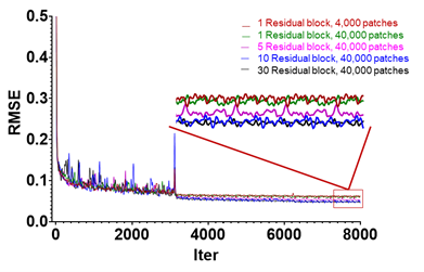
Fig. R1: Training curves of MRH-AF with number of residual blocks ranging from 1 to 30 showing decreasing RMSEs with increasing iterations. The curves in the red rectangular box on the right are enlarged to compare the RMSE values. The training curves of 10 and 30 residual blocks are comparable, both converged with lower RMSE values than the results with 1 and 5 residual blocks.
In addition, the deep learning approach can better accommodate residual mismatches between co-registered histology and MRI than polynomial fitting. Even after careful co-registration, residual mismatches between histology and MRI data can still be found, which pose a challenge for polynomial fittings. We have tested the effect of mismatch by introducing voxel displacements to perfectly co-registered diffusion MRI datasets and demonstrated that the deep learning network used in this study can handle the mismatches (Figure 1 – figure supplement 1).
Relatedly, the comparison between the MRH approach and some standard measures such as FA, MD, and MTR is unfair. Their network is trained to match the histology data, but the standard measures are not. How does the MRH approach compare to e.g. simply combining FA/MD/MTR to map to histology? This to me would be a more relevant comparison.
This is a good idea. We have added maps generated by linear fitting of five MR measures (T2, MTR, FA, MD, and MK) to MBP for a proper comparison. Please see the revised Figure 3A-B. The MRH approach provided better prediction than linear fitting of the five MR measures, as shown by the ROC curves in Figure 3C.
- Not clear if there are 64 layers or 64 residual blocks. Also, is the convolution only doing something across channels? i.e. do we get the same performance by simply averaging the 3x3 voxels?
We have revised the paragraph on the network architecture to clarify this point in Figure 1 caption as well as the Methods section. We used 30 residual blocks, each consists of 2 layers. There are additional 4 layers at the input and output ends, so we had 64 layers in total.
The convolution mostly works across channels, which is what we intended as we are interested in finding the local relationship between multiple MRI contrasts and histology. With inputs from modified 3x3 patches, in which all voxels were assigned the same values as the center voxel, the predictions of MRH-AF did not show apparent loss in sensitivity and specificity, and the voxel-wise correlation with reference AF data remained strong (See Fig. R2 below). We think this is an important piece of information and added it as Figure 1 – figure supplement 3. Averaging the 3x3 voxels in each patch produced similar results.
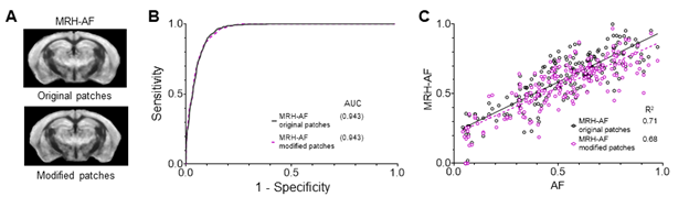
Fig. R2: Evaluation of MRH-AF results generated using modified 3x3 patches with 9 voxels assigned the same MR signals as the center voxel as inputs. A: Visual inspection showed no apparent differences between results generated using original patches and those using modified patches. B: ROC analysis showed a slight decrease in AUC for the MRH-AF results generated using modified patches (dashed purple curve) compared to the original (solid black curve). C: Correlation between MRH-AF using modified patches as inputs and reference AF signals (purple open circles) was slightly lower than the original (black open circles).
The result in the shiverer mouse is most impressive. Were the shiverer mice data included in the training? If not, this should be mentioned/highlighted as it is very cool.
Data from shiverer mice and littermate controls were not included in the training. We have clarified this point in the manuscript.
-
Evaluation Summary:
This paper demonstrates how MRI can be used to mimic histological measures. This is something that the field of MRI has dubbed virtual histology (or MR-histology) for a while, but to my knowledge this paper is the first convincing demonstration that it can be achieved. The paper combines open access mouse histology data from the Allen Institute with their own multimodal post-mortem MRI, and using deep convolutional networks, are able to build models that map MRI data onto multiple histological contrasts. Some of the results are impressive, such as predicting the outcome of histology on mutant shiverer mice.
(This preprint has been reviewed by eLife. We include the public reviews from the reviewers here; the authors also receive private feedback with suggested changes to the manuscript. Reviewer #1 agreed to share …
Evaluation Summary:
This paper demonstrates how MRI can be used to mimic histological measures. This is something that the field of MRI has dubbed virtual histology (or MR-histology) for a while, but to my knowledge this paper is the first convincing demonstration that it can be achieved. The paper combines open access mouse histology data from the Allen Institute with their own multimodal post-mortem MRI, and using deep convolutional networks, are able to build models that map MRI data onto multiple histological contrasts. Some of the results are impressive, such as predicting the outcome of histology on mutant shiverer mice.
(This preprint has been reviewed by eLife. We include the public reviews from the reviewers here; the authors also receive private feedback with suggested changes to the manuscript. Reviewer #1 agreed to share their name with the authors.)
-
Reviewer #1 (Public Review):
Although the results are impressive, the paper has several weaknesses, particularly in terms of analysis, as listed below.
As far as I can tell, the input to the model are raw diffusion data plus a couple of maps extracted from T2 and MT data. While this is ok for the kind of models used here, it means that the networks trained will not generalise to other diffusion protocols (e.g with different bvecs). This greatly reduces to usefulness of this model and hinders transfer to e.g. human data. Why not use summary measures from the data as an input. There are a number of rotationally invariant summary measures that one can extract. I suspect that the first layers of the network may be performing operations such as averaging that are akin to calculating summary measures, so the authors should consider doing that …
Reviewer #1 (Public Review):
Although the results are impressive, the paper has several weaknesses, particularly in terms of analysis, as listed below.
As far as I can tell, the input to the model are raw diffusion data plus a couple of maps extracted from T2 and MT data. While this is ok for the kind of models used here, it means that the networks trained will not generalise to other diffusion protocols (e.g with different bvecs). This greatly reduces to usefulness of this model and hinders transfer to e.g. human data. Why not use summary measures from the data as an input. There are a number of rotationally invariant summary measures that one can extract. I suspect that the first layers of the network may be performing operations such as averaging that are akin to calculating summary measures, so the authors should consider doing that prior to feeding the network.
The noise sensitivity analysis is misleading. The authors add noise to each channel and examine the output, they do this to find which input is important. They find that T2/MT are more important for the prediction of the AF data, But majority of the channels are diffusion data, where there is a lot of redundant information across channels. So it is not surprising that these channels are more robust to noise. In general, the authors make the point that they not only predict histology but can also interpret their model, but I am not sure what to make of either the t-SNE plots or the rose plots. I am not sure that these plots are helping with understanding the model and the contribution of the different modalities to the predictions.
Is deep learning really required here? The authors are using a super deep network, mostly doing combinations of modalities. is the mapping really highly nonlinear? How does it compare with a linear or close to linear mapping (e.e. regression of output onto input and quadratic combinations of input)? How many neurons are actually doing any work and how many are silent (this can happen a lot with ReLU nonlinearities)? In general, not much is done to convince the reader that such a complex model is needed and whether a much simpler regression approach can do the job.
Relatedly, the comparison between the MRH approach and some standard measures such as FA, MD, and MTR is unfair. Their network is trained to match the histology data, but the standard measures are not. How does the MRH approach compare to e.g. simply combining FA/MD/MTR to map to histology? This to me would be a more relevant comparison.
Some details of the modelling is missing (apologies if it's there but I missed it):
- Not clear if there are 64 layers or 64 residual blocks. Also, is the convolution only doing something across channels? i.e. do we get the same performance by simply averaging the 3x3 voxels?
- The result in the shii]verer mouse is most impressive. Were the shiverer mice data included in the traning? If not, this should be mentioned/highlighted as it is very cool. -
Reviewer #2 (Public Review):
The overall idea behind this paper is exciting - use multimodal MRI, co-registered to histology, to train a predictor of a histology image given the MRI input. They demonstrate the potential of this technique using a series of datasets from the Allen Brain Institute, showing decent face validity and further being able to probe which MRI contrasts most contribute to which cellular predictions. The resulting maps of predicted myelin basic protein and predicted Nissl staining appear convincing, lending credibility to the overall effort. Furthermore, the MRI acquisitions and image processing and deep learning steps all seem very well executed.
The most important limitation in this study is, to me, that the MRI and histology samples come from different animals. It is not immediately clear that the prediction …
Reviewer #2 (Public Review):
The overall idea behind this paper is exciting - use multimodal MRI, co-registered to histology, to train a predictor of a histology image given the MRI input. They demonstrate the potential of this technique using a series of datasets from the Allen Brain Institute, showing decent face validity and further being able to probe which MRI contrasts most contribute to which cellular predictions. The resulting maps of predicted myelin basic protein and predicted Nissl staining appear convincing, lending credibility to the overall effort. Furthermore, the MRI acquisitions and image processing and deep learning steps all seem very well executed.
The most important limitation in this study is, to me, that the MRI and histology samples come from different animals. It is not immediately clear that the prediction obtained by comparing different brain areas, which is essential what this prediction will produce, will be accurate in the case of different types of subtle or coarse pathology. As such, this manucript would need ideally a full training set of MRI and histology from the same mice, again ideally consisting of both healthy brains as well as models with pathology. In the absence of such a rich training set at least a strong validation set with histology and MRI in the same animals is needed in order to prove the validity of the proposed method. This does exist, as shown for example for the shiverer mice in Fig 3. Yet the comparison is purely qualitative, with no attempt made to directly quantitate how accurate the predicted histology maps are compared to the real thing, which is a missed opportunity.
There is definitely value to the proposed approach, in particular around understanding which MRI modalities are most likely to contribute to certain cellular staining techniques. The trained networks for different cellular contrasts look intriguing. Yet without samples from the same animal directly and quantitatively compared the results cannot be clearly evaluated.
-
